Implicit Feature Detection via a Constrained Topic Model and SVM

Implicit Feature Detection via a Constrained Topic Model and SVM

Wei Wang

, Hua Xu

and

Xiaoqiu Huang

∗

_{State Key Laboratory of Intelligent Technology and Systems,}

Tsinghua National Laboratory for Information Science and Technology,

Department of Computer Science and Technology, Tsinghua University,

Beijing 100084, China

†

_{Beijing University of Posts and Telecommunications, Beijing 100876, China}

[email protected], [email protected], [email protected]

Abstract

Implicit feature detection, also known as im-plicit feature identification, is an essential as-pect of feature-specific opinion mining but previous works have often ignored it. We think, based on the explicit sentences, sever-al Support Vector Machine (SVM) classifier-s can be eclassifier-stabliclassifier-shed to do thiclassifier-s taclassifier-sk. Never-theless, we believe it is possible to do bet-ter by using a constrained topic model instead of traditional attribute selection methods. Ex-periments show that this method outperforms the traditional attribute selection methods by a large margin and the detection task can be completed better.

1

Introduction

Feature-specific opinion mining has been well de-fined by Ding and Liu(2008). Example 1 is a cell phone review in which two features are mentioned.

Example 1 This cell phone is fashion in

appear-ance, and it is also very cheap.

If a feature appears in a review directly, it is called anexplicit feature. If a feature is only implied, it is

called animplicit feature. In Example 1,appearance

is an explicit feature whilepriceis an implicit

fea-ture, which is implied bycheap. Furthermore, an

ex-plicit sentenceis defined as a sentence containing at

least one explicit feature, and animplicit sentenceis

the sentence only containing implicit features. Thus, the first sentence is an explicit sentence, while the second is an implicit one.

This paper proposes an approach for implicit fea-ture detection based on SVM and Topic Model(TM).

The Topic Model, which incorporated into con-straints based on the pre-defined product feature, is established to extract the training attributes for SVM. In the end, several SVM classifiers are con-structed to train the selected attributes and utilized to detect the implicit features.

2

Related Work

The definition of implicit feature comes from Liu et al. (2005)’s work. Su et al. (2006) used Point-wise Mutual Information (PMI) based semantic as-sociation analysis to identify implicit features, but no quantitative experimental results were provided. Hai et al. (2011) used co-occurrence association rule mining to identify implicit features. However, they only dealt with opinion words and neglected the facts. Therefore, in this paper, both the opinions and facts will be taken into account.

Blei et al. (2003) proposed the original LDA us-ing EM estimation. Griffiths and Steyvers (2004) applied Gibbs sampling to estimate LDA’s parame-ters. Since the inception of these works, many vari-ations have been proposed. For example, LDA has previously been used to construct attributes for clas-sification; it often acts to reduce data dimension(Blei and Jordan, 2003; Fei-Fei and Perona, 2005; Quel-has et al., 2005). Here, we modify LDA and adopt it to select the training attributes for SVM.

3

Model Design

3.1 Introduction to LDA

We briefly introduce LDA, following the notation

of Griffiths(Griffiths and Steyvers, 2004). GivenD

documents expressed over W unique words and T

topics, LDA outputs the document-topic distribution

θ and topic-word distributionφ, both of which can

be obtained with Gibbs Sampling. For this scheme, the core process is the topic updating for each word in each document according to Equation 1.

P(zi=j|z−i,w, α, β) =

( n

(wi)

−i,j+β

∑W w′n

(w′)

−i,j+W β

)( n

(di)

−i,j+α

∑T j n

(di)

−i,j+T α

) (1)

wherezi = j represents the assignment of theith

word in a document to topic j, z₋i represents all

the topic assignments excluding theithword. n(_jw′)

is the number of instances of word w′ assigned to

topicj andn(di)

j is the number of words from

doc-ument di assigned to topicj, the−i notation

sig-nifies that the counts are taken omitting the value

of zi. Furthermore, α and β are hyper-parameters

for the document-topic and topic-word Dirichlet dis-tributions, respectively. After N iterations of Gibbs sampling for all words in all documents, the

distri-butionθandφare finally estimated using Equations

2 and 3.

ϕ(wi)

j =

n(wi)

j +β

∑W w′n

(w′)

j +W β

(2)

θ(di)

j =

n(di)

j +α

∑T j n

(di)

j +T α

(3)

3.2 Framework

Algorithm 1 summarizes the main steps. When a specific product and the reviews are provided, the explicit sentences and corresponding features are extracted(Line 1) by word segmentation, part-of-speech(POS) tagging and synonyms feature cluster-ing. Then the prior knowledge are drawn from the explicit sentences automatically and integrated in-to the constrained in-topic model((Line 3 - Line 5). The word clusters are chosen as the training at-tributes(Line 6). Finally, several SVM classifier-s are generated and applied to detect implicit fea-tures(Line 7 - Line 12).

Algorithm 1Implicit Feature Detection

1: ES←extract explicit sentence set 2: N ES←non-explicit sentence set 3: CS←constraint set fromES

4: CP K←correlation prior knowledge fromES

5: ET M←ConstrainedTopicModel(T,ES,CS,CP K) 6: T A←select training attributes fromET M

7: foreachfiin feature clustersdo

8: T Di←GenerateTrainingData(T Ai,ES)

9: Ci←BuildClassificationModelBySVM(T Di)

10: P Ri←positive result of Classify(Ci,N ES)

11: the feature of sentence inP Ri←fi

12: end for

3.3 Prior Knowledge Extraction and

Incorporation

It is obvious that the pre-existing knowledge can as-sist to produce better and more significant clusters. In our work, we use a constrained topic model to s-elect attributes for each product features. Each topic is first pre-defined a product feature. Then two type-s of prior knowledge, which are derived from the pre-defined product features, are extracted automat-ically and incorporated: must-link/cannot-link and correlation prior knowledge.

3.3.1 Must-link and Cannot-link

Must-link: It specifies that two data instances must be in the same cluster. Here is the must-link

from an observation: as ”cheap” to ”price”, some

words must be associated with a feature. In order to mine these words, we compute the co-occurrence

degree byfrequency*PMI(f,w), whose formula is as

following:Pf&w∗log2

Pf&w

PfPw, whereP is the

proba-bility of subscript occurrence in explicit sentences,

f is the feature, w is the word, and f&w means

the co-occurrence of f and w. A higher value of

frequency*PMI signifies that w often indicates f.

For a feature fi, the top five words and fi

consti-tute must-links. For example, the co-occurrence of ”price” and ”cheap” is very high, then the must-link

between ”price” and ”cheap” can be identified.

Cannot-link: It specifies that two data instances cannot be in the same cluster. If a word and a fea-ture never co-occur in our corpus, we assume them

to form a cannot-link. For example, the word

low-costhas never co-occurred with the product feature

cor-pus.

In this paper, the pre-defined process, must-link, and cannot-link are derived from Andrzejewski and Zhu (2009)’s work, all must-links and cannot-links are incorporated our constrained topic model. We

multiply an indicator functionδ(wi, zj), which

rep-resents a hard constraint, to the Equation 1 as the final probability for topic updating (see Equation 4).

P(zi =j|z−i,w, α, β) =

δ(wi, zj)(

n(wi)

−i,j+β

∑W w′n

(w′)

−i,j+W β

)( n

(di)

−i,j+α

∑T j n

(di)

−i,j+T α

)

(4)

As illustrated by Equations 1 and 4, δ(wi, zj),

which represents intervention or help from pre-existing knowledge of must-links and cannot-links, plays a key role in this study. In the topic updating for each word in each document, we assume that the

current word iswiand its linked feature topic set is

Z(wi)_{, then for the current topicz}

j,δ(wi, zj)is

cal-culated as follows:

1. If wi is constrained by must-links and the

linked feature belongs toZ(wi)_,δ(w

i, zj|zj ∈

Z(wi)_{) = 1andδ(w}

i, zj|zj ∈/Z(wi)) = 0.

2. If wi is constrained by cannot-links and the

linked feature belongs toZ(wi)_,δ(w

i, zj|zj ∈

Z(wi)_{) = 0andδ(w}

i, zj|zj ∈/Z(wi)) = 1.

3. In other cases,δ(wi, zj|j= 1, . . . , T) = 1.

3.3.2 Correlation Prior Knowledge

In view of the explicit product feature of each top-ic, the association of the word and the feature to topic-word distribution should be taken into accoun-t. Therefore, Equation 2 is revised as the following:

ϕ(wi)

j =

(1 +Cwi,j)(n

(wi)

j ) +β

∑W

w′(1 +Cw′,j)(n

(w′)

j ) +W β

(5)

where Cw′,j reflects the correlation ofw′ with the

topicj, which is centered on the product featurefzj.

The basic idea is to determine the association ofw′

andfzj, if they have the high relevance,Cw′,jshould

be set as a positive number. Otherwise, if we can

determinew′ andfzj are irrelevant,Cw′,j should be

set as a positive number. In this paper, we attempt to using PMI or dependency relation to judge the

relevance. For wordw′and featurefzj:

1. Dependency relation judgement: If w′ as

par-ent node in the syntax tree mainly co-occurs

withfzj,Cw′,jwill be set positive. Ifw′mainly

co-occurs with several features including fzj,

Cw′,j will be set negative. Otherwise, Cw′,j

will be set 0.

2. PMI judgement: If w′ mainly co-occurs with

fzj andP M I(w′, fzj) is greater than the

giv-en value,Cw′,j will be set positive. Otherwise,

Cw′,j will be set negative.

3.4 Attribute Selection

Some words, such as ”good”, can modify

sever-al product features and should be removed. In the result of run once, if a word appears in the topics which relates to different features, it is defined as a conflicting word. If a term is thought to describe several features or indicate no features, it is defined

as anoise word.

When each topic has been pre-allocated, we run the explicit topic model 100 times. If a word turns

into a conflicting wordTcw times(Tcw is set to 20),

we assume that it is a noise word. Then the noise word collection is obtained and applied to filter the explicit sentences. Actually, here 100 is just an

esti-mated number. And forTcw, when it is between 15

and 25, the result is same, and when it exceeds 25, the result does not change a lot. The most important part to filter noise words is the correlation compu-tation. So the experiment can work well with only estimated parameters.

Next, By integrating pre-existing knowledge, the

explicit topic model, which runsTiter times,

sever-s asever-s attribute sever-selection for SVM. In every resever-sult for each topic cluster, we remove the least four prob-able of word groups and merge the results by the pre-defined product feature. For a feature, if a word

appears in its topic words more than Titer ∗tratio

0 10 20 30 40 50 60 70 80 90 100

Attribute Factor Number ChiSquare GainRatio InfoGain

(a) SVM based on traditional attribute selection method

0.0 0.1 0.2_t 0.3 0.4 0.5

ratio TM TM+must TM+cannot TM+must+cannot TM+syntactic TM+must+cannot+syntactic TM+PMI TM+must+cannot+PMI TM+correlation knowledge(PMI+syntactic) TM+must+cannot+correlation knowledge

(b) our constrained topic model by differenttratio(Titer= 20)

0 10 20 T iter30 40 50

TM TM+must TM+cannot TM+must+cannot TM+syntactic TM+must+cannot+syntactic TM+PMI TM+must+cannot+PMI TM+correlation knowledge(PMI+syntactic) TM+must+cannot+correlation knowledge

(c) our constrained topic model by differentTiter(tratio= 0.1)

Figure 1: Performance of different cases

3.5 Implicit Feature Detection via SVM

After completing attribute selection, vector space model(VSM) is applied to the selected attributes on

the explicit sentences. For each featurefi, a SVM

classifierCiis adopted. In train-set, the positive

cas-es are the explicit sentenccas-es offi, and the negative

cases are the other explicit sentences. For a

non-explicit sentence, if the classification result ofCiis

positive, it is an implicit sentence which impliesfi.

4

Evaluation of Experimental Results

4.1 Data Sets

There has no standard data set yet, we crawled the experiment data, which included reviews about a cellphone, from a famous Chinese shopping

web-site1. The data contains 14218 sentences. The

fea-ture of each sentence was manually annotated by

two research assistants. A handful of sentences

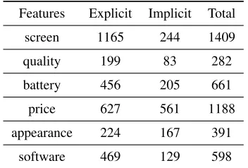
which were annotated inconsistently were deleted. Table 1 depicts the data set which is evaluated. Other features were ignored because of their rare appear-ance.

Here are some explanations: (1)The sentences

containing several explicit features were not added

to the train-set.(2)A tiny number of sentences

con-tain both explicit and implicit features, and they can

only be regarded as explicit sentences.(3)The

train-ing set contains 3140 explicit sentences, the test set contains 7043 non-explicit sentences and more than

5500 sentences have no feature. (4) According to

the ratio among the explicit sentences(6:1:2:3:1:2), it is reasonable that the most suitable number of top-ics should be 14. For example, the ratio of the

prod-1_{http://www.360buy.com/}

Table 1: Experiment data

Features Explicit Implicit Total

screen 1165 244 1409

quality 199 83 282

battery 456 205 661

price 627 561 1188

appearance 224 167 391

software 469 129 598

uct featurescreenis 6, so we can assign the feature

to topic 0,1,2,3,4,5. In our experiment, the perfor-mance of algorithm 1 is evaluated using F-measure.

(5)Although the size of dataset is limited, out

pro-posed is based on the constraint-based topic model, which has been widely used in different NLP field-s. So, our approach can generalize well in different datasets. Of course, more high quality data will be collected to do the experiment in the future.

4.2 Experimental Results

Figure 1a depicts the performance of using tradi-tional attribute selection methods on SVM. Using

χ2 teston SVM can achieve the best performance,

which is about 66.7%. In our constrained topic

model, we use different Titer and tratio. We

con-ducted experiments by incorporating different types prior knowledge. From Figure 1b and 1c, we

con-clude that:(1)All these methods perform much

bet-ter than the traditional feature selection methods, the

improvements are more than 6%. (2)The reason for

word-s. (3)All the pre-existing knowledge performs best and shows 3% improvement over non prior

knowl-edge. (4)Different types of prior knowledge have

different impact on the stabilities of different

pa-rameters. (5)As we have expected, by combing

al-l prior knowal-ledge, the best performance can reach

77.78%. Furthermore, as tratio or Titer changes,

our constrained topic model incorporating all prior knowledge look like very stable.

5

Conclusions

In this paper, we adopt a constrained topic model incorporating prior knowledge to select attribute for SVM classifiers to detect implicit features. Exper-iments show this method outperforms the attribute feature selection methods and detect implicit fea-tures better.

6

Acknowledgments

This work is supported by National Natural Science Foundation of China (Grant No: 61175110) and Na-tional Basic Research Program of China (973 Pro-gram, Grant No: 2012CB316305).

References

David Andrzejewski and Xiaojin Zhu. 2009. Laten-t dirichleLaten-t allocaLaten-tion wiLaten-th Laten-topic-in-seLaten-t knowledge. In Proceedings of the NAACL HLT 2009 Workshop on Semi-Supervised Learning for Natural Language Pro-cessing, pages 43–48. Association for Computational Linguistics.

D.M. Blei and M.I. Jordan. 2003. Modeling annotated data. InProceedings of the 26th annual international ACM SIGIR conference on Research and development in informaion retrieval, pages 127–134. ACM. D.M. Blei, A.Y. Ng, and M.I. Jordan. 2003.

Laten-t dirichleLaten-t allocaLaten-tion.the Journal of machine Learning research, 3:993–1022.

Xiaowen Ding, Bing Liu, and Philip S. Yu. 2008. A holistic lexicon-based approach to opinion mining. In Proceedings of the international conference on Web search and web data mining, WSDM ’08, pages 231– 240, New York, NY, USA. ACM.

L. Fei-Fei and P. Perona. 2005. A bayesian hierarchical model for learning natural scene categories. In Com-puter Vision and Pattern Recognition, 2005. CVPR 2005. IEEE Computer Society Conference on, vol-ume 2, pages 524–531. IEEE.

T.L. Griffiths and M. Steyvers. 2004. Finding scientif-ic topscientif-ics. Proceedings of the National Academy of Sciences of the United States of America, 101(Suppl 1):5228–5235.

Z. Hai, K. Chang, and J. Kim. 2011. Implicit feature identification via co-occurrence association rule min-ing. Computational Linguistics and Intelligent Text Processing, pages 393–404.

B. Liu, M. Hu, and J. Cheng. 2005. Opinion observer: analyzing and comparing opinions on the web. In Pro-ceedings of the 14th international conference on World Wide Web, pages 342–351. ACM.

P. Quelhas, F. Monay, J.M. Odobez, D. Gatica-Perez, T. Tuytelaars, and L. Van Gool. 2005. Modeling scenes with local descriptors and latent aspects. In Computer Vision, 2005. ICCV 2005. Tenth IEEE In-ternational Conference on, volume 1, pages 883–890. IEEE.