Training Connectionist Models for the Structured Language Model

Training Connectionist Models for the Structured Language Model

Peng Xu, Ahmad Emami and Frederick Jelinek

Center for Language and Speech Processing Johns Hopkins University

Baltimore, MD 21218

xp,emami,jelinek @jhu.edu

Abstract

We investigate the performance of the Structured Language Model (SLM) in terms of perplexity (PPL) when its compo-nents are modeled by connectionist mod-els. The connectionist models use a dis-tributed representation of the items in the history and make much better use of contexts than currently used interpolated or back-off models, not only because of the inherent capability of the connection-ist model in fighting the data sparseness problem, but also because of the sub-linear growth in the model size when the context length is increased. The connec-tionist models can be further trained by an EM procedure, similar to the previously used procedure for training the SLM. Our experiments show that the connectionist models can significantly improve the PPL over the interpolated and back-off mod-els on the UPENN Treebank corpora, after interpolating with a baseline trigram lan-guage model. The EM training procedure can improve the connectionist models fur-ther, by using hidden events obtained by the SLM parser.

1 Introduction

In many systems dealing with natural speech or lan-guage such as Automatic Speech Recognition and

This work was supported by the National Science Founda-tion under grants No.IIS-9982329 and No.IIS-0085940.

Statistical Machine Translation, a language model is a crucial component for searching in the often prohibitively large hypothesis space. Most of the state-of-the-art systems use n-gram language mod-els, which are simple and effective most of the time. Many smoothing techniques that improve lan-guage model probability estimation have been pro-posed and studied in the n-gram literature (Chen and Goodman, 1998).

Recent efforts have studied various ways of us-ing information from a longer context span than that usually captured by normal n-gram language mod-els, as well as ways of using syntactical informa-tion that is not available to the word-based n-gram models (Chelba and Jelinek, 2000; Charniak, 2001; Roark, 2001; Uystel et al., 2001). All these language models are based on stochastic parsing techniques that build up parse trees for the input word sequence and condition the generation of words on syntactical and lexical information available in the parse trees. Since these language models capture useful hierar-chical characteristics of language, they can improve the PPL significantly for various tasks. Although more improvement can be achieved by enriching the syntactical dependencies in the structured language model (SLM) (Xu et al., 2002), a severe data sparse-ness problem was observed in (Xu et al., 2002) when the number of conditioning features was increased.

with the number of predicting features used. It has been shown that this method improves significantly on regular n-gram models in perplexity (Bengio et al., 2001). The ability of the method to accommo-date longer contexts is most appealing, since exper-iments have shown consistent improvements in PPL when the context of one of the components of the SLM is increased in length (Emami et al., 2003). Moreover, because the SLM provides an EM train-ing procedure for its components, the connectionist models can also be improved by the EM training.

In this paper, we will study the impact of neural network modeling on the SLM, when all of its three components are modeled with this approach. An EM training procedure will be outlined and applied to further training of the neural network models.

2 A Probabilistic Neural Network Model

Recently, a relatively new type of language model has been introduced where words are represented by points in a multi-dimensional feature space and the probability of a sequence of words is computed by means of a neural network. The neural network, having the feature vectors of the preceding words as its input, estimates the probability of the next word (Bengio et al., 2001). The main idea behind this model is to fight the curse of dimensionality by inter-polating the seen sequences in the training data. The generalization this model aims at is to assign to an unseen word sequence a probability similar to that of a seen word sequence whose words are similar to those of the unseen word sequence. The similarity is defined as being close in the multi-dimensional space mentioned above.

In brief, this model can be described as follows. A feature vector is associated with each token in the

input vocabulary, that is, the vocabulary of all the

items that can be used for conditioning. Then the conditional probability of the next word is expressed as a function of the input feature vectors by means of a neural network. This probability is produced for every possible next word from the output

vocab-ulary. In general, there does not need to be any

rela-tionship between the input and output vocabularies. The feature vectors and the parameters of the neural network are learned simultaneously during training. The input to the neural network are the feature

vec-tors for all the inputs concatenated, and the output is the conditional probability distribution over the output vocabulary. The idea here is that the words which are close to each other (close in the sense of their role in predicting words to follow) would have similar (close) feature vectors and since the proba-bility function is a smooth function of these feature values, a small change in the features should only lead to a small change in the probability.

2.1 The Architecture of the Neural Network Model

The conditional probability function

where and

are from the input and output vocabularies

and respectively, is determined in two parts:

1. A mapping that associates with each word in the input vocabulary

a real vector of fixed length

2. A conditional probability function which takes as the input the concatenation of the feature vectors of the input items

. The function produces a probability distribu-tion (a vector) over , the "!$# element being the conditional probability of the %!$# member of . This probability function is realized by a standard multi-layer neural network. A

soft-max function (Equation 4) is used at the output

of the neural net to make sure probabilities sum to 1.

Training is achieved by searching for parameters

&

of the neural network and the values of feature vectors that maximize the penalized log-likelihood of the training corpus:

')(+* ,-/.10

3254687 .:9;.

*$<>=>=>=>< ;.?@

*:ABDC E

6

BDC (1)

whereGF5F

HIHIHI F

is the probability of word F

(network output at time!),J is the training data size and K

L&M

is a regularization term, sum of the parameters’ squares in our case.

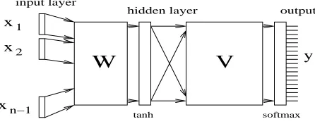
x₁ x₂ x_n−1 output hidden layer input layer

W

V

Figure 1: The neural network architecture

make sure that the scores are positive and sum up to one, hence are valid probabilities. More specifically, the output of the hidden layer is given by:

( 6 ? @ * * C ( <

<>=>=>=< (2) where #

is the

!# output of the hidden layer, !

is the" !# input of the network, #

and

$

are weight and bias elements for the hidden layer respectively, and% is the number of hidden units.

Furthermore, the outputs are given by:

& ( - (' ) ( < <>=>=>=< 9 ' ) 9 (3) * 5( +, + , ( < <>=>=>=< 9 ' ) 9 (4) where and $

are weight and bias elements for the output layer before the softmax layer. The soft-max layer (equation 4) ensures that the outputs are positive and sum to one, hence are valid probabili-ties. The !$# output of the neural network, corre-sponding to the !$# item

of the output vocab-ulary, is exactly the sought conditional probability, that is

-/.

F

.

F HIHIHI F .

2.2 Training the Neural Network Model

Standard back-propagation is used to train the pa-rameters of the neural network as well as the feature vectors. See (Haykin, 1999) for details about neural networks and back-propagation. The function we try to maximize is the log-likelihood of the training data given by equation 1. It is straightforward to com-pute the gradient of the likelihood function for the feature vectors and the neural network parameters, and hence compute their updates.

We should note from equation 4 that the neural network model is similar in functional form to the maximum entropy model (Berger et al., 1996) ex-cept that the neural network learns the feature func-tions by itself from the training data. However,

unlike the G/IIS algorithm for the maximum en-tropy model, the training algorithm (usually stochas-tic gradient descent) for the neural network models is not guaranteed to find even a local maximum of the objective function.

It is very important to mention that one of the great advantages of this model is that the number of inputs can be increased causing only sub-linear increase in the number of model parameters, as op-posed to exponential growth in n-gram models. This makes the parameter estimation more robust, espe-cially when the input span is long.

3 Structured Language Model

An extensive presentation of the SLM can be found in (Chelba and Jelinek, 2000). The model assigns a probability

#

0%

to every sentence # and ev-ery possible binary parse 0

. The terminals of 0 are the words of # with POS tags, and the nodes of0

are annotated with phrase headwords and non-terminal labels. Let # be a sentence of length 1

(<s>, SB) ... (w_p, t_p) (w_{p+1}, t_{p+1}) ... (w_k, t_k) w_{k+1}.... </s> h_0 = (h_0.word, h_0.tag)

h_{-1} h_{-m} = (<s>, SB)

Figure 2: A word-parse -prefix

words to which we have prepended the sentence be-ginning marker<s>and appended the sentence end marker</s>so that 243

.

<s>and2

. </s>. Let # 5. 263 HHH 2

be the word

-prefix of the sentence — the words from the beginning of the sentence up to the current position — and #

0

the word-parse -prefix. Figure 2 shows a word-parse -prefix; h_0, .., h_{-m} are the

ex-posed heads, each head being a pair (headword,

non-terminal label), or (word, POS tag) in the case of a root-only tree. The exposed heads at a given po-sition in the input sentence are a function of the word-parse -prefix.

3.1 Probabilistic Model

The joint probability

#

0%

of a word sequence

# and a complete parse

0

can be broken up into:

46 <7C ( 8 ?9 * *: 46<; 9 @ * 7 @ * C>= 46 F 9 @ * 7 @ * < ; C?= 8A@ B< * 46 * B 9 @ * 7 @ * < ; < F < * * =>=>= * B @

where: # 0

is the word-parse

" -prefix 2

is the word predicted by WORD-PREDICTOR

!

is the tag assigned to

2

by the TAGGER

is the number of operations the CON-STRUCTOR executes at sentence position before passing control to the WORD-PREDICTOR (the

-th operation at position k is the

null transi-tion);

is a function of

0

denotes the -th CONSTRUCTOR operation carried out at position k in the word string; the op-erations performed by the CONSTRUCTOR ensure that all possible binary branching parses, with all possible headword and non-terminal label assign-ments for the2

HHH

2

word sequence, can be gen-erated. The

HHH

sequence of CONSTRUC-TOR operations at position grows the word-parse

"

-prefix into a word-parse -prefix.

The SLM is based on three probabilities, each can be specified using various smoothing methods and parameterized (approximated) by using differ-ent contexts. The bottom-up nature of the SLM parser enables us to condition the three probabili-ties on features related to the identity of any exposed head and any structure below the exposed head. Since the number of parses for a given word prefix

#

grows exponentially with , !0 , the state space of our model is huge even for rela-tively short sentences, so we have to use a search strategy that prunes it. One choice is a synchronous multi-stack search algorithm (Chelba and Jelinek, 2000) which is very similar to a beam search.

The language model probability assignment for the word at position

in the input sentence is made using: 4 6<; 9 * 9 C . - 46<; 9 * 9 7 C?= 6 <7 C< 6 <7 C . 46 7 C - 46 7

C < (6) which ensures a proper probability normalization over strings # , where

is the set of all parses present in our stacks at the current stage .

3.2 N-best EM Training of the SLM

Each model component of the SLM —WORD-PREDICTOR, TAGGER, CONSTRUCTOR— is initialized from a set of parsed sentences after under-going headword percolation and binarization. An N-best EM (Chelba and Jelinek, 2000) variant is then

employed to jointly reestimate the model parameters such that the PPL on training data is decreased — the likelihood of the training data under our model is increased. The reduction in PPL is shown experi-mentally to carry over to the test data.

Let

#

0

denote the joint sequence of # with parse structure 0

. The probability of a

# 0% se-quence # 0

is, according to Equation 5, the product of the corresponding elementary events. This product form makes the three components of the SLM separable, therefore, we can estimate the parameters separately. According to the EM algo-rithm, the auxiliary function can be written as:

6"! <$# ! C ( -% 46 7 9 A$# ! C 0 32546 <7A !

C= (7) The E step in the EM algorithm is to find

0

#'&)( *

under the model parameters (

*

of the previous iteration, the M step is to find parame-ters

*

that maximize the auxiliary function+ *

(

* above. In practice, since the space of0

, all possi-ble parses, is huge, we normally use a synchronous multi-stack search algorithm to sample the most probable

parses and approximate the space by the N-best parses. (Chelba and Jelinek, 2000) showed that as long as the N-best parses remain invariant, the M step will increase the likelihood of the train-ing data.

4 Neural Network Models in the SLM

As described in the previous section, the three com-ponents of the SLM can be parameterized in various ways. The neural network model, because of its abil-ity in fighting the data sparseness problem, is a very natural choice when we want to use longer contexts to improve the language model performance.

The training criterion for the neural network model is given by Equation 1 , when we have la-beled training data for the SLM. The labels —the parse structure— are used to get the conditioning variables. In order to take advantage of the ability of the SLM in generating many hidden parses, we need to modify the training criterion for the neural network model. Actually, if we take the EM auxil-iary function in Equation 7 and find parameters of the neural network models to maximize +

*

(

the derivative of with respect to the parameters is calculated and used as the direction for the gra-dient descent algorithm. Since +

*

(

*

is nothing but a weighted average of the log-likelihood func-tions, the derivative of + with respect to the param-eters is then a weighted average of the derivatives of the log-likelihood functions. In practice, we use the SLM with all components modeled by neural net-works to generate N-best parses in the E step, and for the M step, we use the modified back-propagation algorithm to estimate the parameters of the neural network models based on the weights calculated in the E step.

We should be aware that there is no proof that this EM procedure can actually increase the likelihood of the training data. Not only are we using a small portion of the entire hidden parse space, but we also use the stochastic gradient descent algorithm that is not guaranteed to converge, for training the neural network models. Bearing this in mind, we will show experimentally that this flawed EM procedure can still lead to improvements in PPL.

5 Experiments

We have used the UPenn Treebank portion of the WSJ corpus to carry out our experiments. The UPenn Treebank contains 24 sections of hand-parsed sentences. We used section 00-20 for training our models, section 21-22 for tuning some param-eters (i.e., estimating discount constant for smooth-ing, and/or making sure overtraining does not occur) and section 23-24 to test our models. Before car-rying out our experiments, we normalized the text in the following ways: numbers in Arabic form are replaced by a single token “N”, punctuations are re-moved, all words are mapped to lower case, extra in-formation in the parse (such like traces) are ignored. The word vocabulary contains 10k words including a special token for unknown words. There are 40 items in the part-of-speech set and 54 items in the non-terminal set, respectively. All of the experimen-tal results in this section are based on this corpus and split, unless otherwise stated.

5.1 Getting a Better Baseline

Since better performance of the SLM was reported recently in (Kim et al., 2001) by using Kneser-Ney

smoothing, we first improved the baseline model by using a variant of Kneser-Ney smoothing: the in-terpolated Kneser-Ney smoothing as in (Goodman, 2001), which is also implemented in the SRILM toolkit (Stolcke, 2002).

There are three notable differences in our imple-mentation of the interpolated Kneser-Ney smooth-ing related to that in the SRILM toolkit. First, we used one discount constant for each n-gram level, in-stead of three different discount constants. Second, our discount constant was estimated by maximizing the log-likelihood of the heldout data (assuming the discount constant is between 0 and 1), instead of the Good-Turing estimate. Finally, in order to deal with the fractional counts we encounter during the EM training procedure, we developed an approxi-mate Kneser-Ney smoothing for fractional counts. For lack of space, we do not go into the details of this approximation, but our approximation becomes the exact Kneser-Ney smoothing when the counts are in-tegers.

In order to test our Kneser-Ney smoothing im-plementation, we built a trigram language model and compared the performance with that from the SRILM. Our PPL was 149.6 and the SRILM PPL was 148.3, therefore, although there are differences in the implementation details, we think our result is close enough to the SRILM.

Having tested the smoothing method, we applied it to the SLM. We used the Kneser-Ney smooth-ing to all components with the same parameteriza-tion as the h-2 scheme in (Xu et al., 2002). Table 1 is the comparison between the deleted-interpolation (DI) smoothing and the Kneser-Ney (KN) smooth-ing. The in Table 1 is the interpolation weight between the SLM and the trigram language model ( =1.0 being the trigram language model). The no-tation “En” indicates the models were obtained af-ter “n” iaf-terations of EM training1. Since Kneser-Ney smoothing is consistently better than deleted-interpolation, we later on report only the Kneser-Ney smoothing results when comparing to the neural network models.

1

Model =0.0 =0.4 =1.0 KN-E0 143.5 132.3 149.6 KN-E3 140.7 131.0 149.6 DI-E0 161.4 149.2 166.6 DI-E3 159.4 148.2 166.6

Table 1: Comparison between KN and DI smoothing

5.2 Training Neural Network Models with the Treebank

We used the neural network models for all of the three components of the SLM. The neural network models are exactly as described in Section 2.1. Since the inputs to the networks are always a mixture of words and NT/POS tags, while the output probabili-ties are over words in the PREDICTOR, POS tags in the TAGGER, and adjoint actions in the PARSER, we used separate input and output vocabularies in all cases. In all of our experiments with the neu-ral network models, we used 30 dimensional feature vectors as input encoding of the mixed items, 100 hidden units and a starting learning rate of 0.001. Stochastic gradient descent was used for training the models for a maximum of 50 iterations. The initial-ization for the parameters is done randomly with a uniform distribution centered at zero.

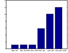
In order to study the behavior of the SLM when longer context is used for conditioning the probabilities, we gradually increased the context of the PREDICTOR model. First, the third exposed previous head was added. Since the syntactical head gets the head word from one of the children, either left or right, the child that does not contain the head word (hence called opposite child) is never used later on in predicting. This is particularly not appropriate for the prepositional phrase because the preposition is always the head word of the phrase in the UPenn Treebank annotation. Therefore, we also added the opposite child of the first exposed previous head into the context for predicting. Both Kneser-Ney smoothing and the neural network model were studied when the context was gradually increased. The results are shown in Table 2.

In Table 2, “nH” stands for “n” exposed previous heads are used for conditioning in the PREDICTOR component, “nOP” stands for “n” opposite children are used, starting from the most recent one. As we can see, when the length of the context is increased,

Model +3gram

KN-2H 143.5 132.3 KN-3H 140.2 128.8 KN-3H-1OP 139.4 129.0 NN-2H 162.4 122.9 NN-3H 156.7 120.3 NN-3H-1OP 151.2 118.4

Table 2: Comparison between KN and NN (E0)

Kneser-Ney smoothing saturates quickly and could not improve the PPL further. On the other hand, the neural network model can still consistently im-prove the PPL, as longer context is used for predict-ing. Overall, the best neural network model (after interpolation with a trigram) achieved 8% relative improvement over the best result from Kneser-Ney smoothing.

Another interesting result is that it seems the neu-ral network model can learn a probability distribu-tion that is less correlated to the normal trigram model. Although before interpolating with the tri-gram, the PPL results of the neural network models are not as good as the Kneser-Ney smoothed models, they become much better when combined with the trigram. In the results of Table 2, the trigram model is a Kneser-Ney smoothed model that gave PPL of 149.6 by itself. The interpolation weight with the tri-gram is 0.4 and 0.5 respectively, for the Kneser-Ney smoothed SLM and neural network based SLM.

0 2 4 6 8 10 12 14

NN−2H NN−3H NN−3H−1OP KN−2H KN−3H KN−3H−1OP

that for the Kneser-Ney smoothed models. Further-more, as the length of context increases, the ratio for the Kneser-Ney smoothed model becomes greater — a clear sign of over-parameterization. However, the ratio for the neural network model changes very little even when the length of the context increases from 4 (2H) to 8 (3H-1OP). The exact reason why the neural network models are more uncorrelated to the trigram is not completely understood, but we conjecture that part of the reason is that the neural network models can learn a probability distribution very different from the trigram by putting much less probability mass on the training examples.

5.3 Training the Neural Network Models with EM

After the neural network models were trained from the labeled data —the UPenn Treebank— we per-formed one iteration of the EM procedure described in Section 4. The neural network model based SLM was used to get N-best parses for each training sen-tence, via the multi-stack search algorithm. This E step provided us a bigger collection of parse struc-tures with weights associated with them. In the next M step, we used the stochastic gradient descent al-gorithm (modified to utilize the weights associated with each parse structure) to train the neural network models. The modified stochastic gradient descent al-gorithm was run for a maximum of 30 iterations and the initial parameter values are those from the the previous iteration.

+3gram NN-3H-1OP E0 151.2 118.4 NN-3H-1OP E1 147.9 117.9 KN-3H-1OP E0 139.4 129.0 KN-3H-1OP E1 139.2 129.2

Table 3: EM training results

Table 3 shows the PPL results after one EM train-ing iteration for both the neural network models and the approximated Kneser-Ney smoothed mod-els, compared to the results before EM training. For the neural network models, the EM training did improve the PPL further, although not a lot. The improvement from training is consistent with the training results showed in (Xu et al., 2002) where deleted-interpolation smoothing was used for the

SLM components. It is worth noting that the ap-proximated Kneser-Ney smoothed models could not improve the PPL after one iteration of EM training. One possible reason is that in order to apply Kneser-Ney smoothing to fractional counts, we had to ap-proximate the discounting. The approximation may degrade the benefit we could have gotten from the EM training. Similarly, the M step in the EM proce-dure for the neural network models also has the same problem: the stochastic gradient descent algorithm

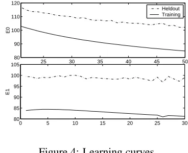
is not guaranteed to converge. This can be clearly

seen in Figure 4 in which we plot the learning curves of the 3H-1OP model (PREDICTOR component) on both training and heldout data at EM iteration 0 and iteration 1. For EM iteration 0, because we started from parameters drawn from a uniform distribution, we only plot the last 30 iterations of the stochastic gradient descent.

25 30 35 40 45 50

80 90 100 110 120

E0

Heldout Training

0 5 10 15 20 25 30

80 85 90 95 100 105

E1

Figure 4: Learning curves

As we expected, the learning curve of the train-ing data in EM iteration 1 is not as smooth as that in EM iteration 0, and even more so for the heldout data. However, the general trend is still decreasing. Although we can not prove that the EM training of the neural network models via the SLM can improve the PPL, we observed experimentally a gain that is favorable comparing to that from the usual Kneser-Ney smoothed models or deleted interpolation mod-els.

6 Conclusion and Future Work

SLM. Overall, the best studied model gave a 21% relative reduction in PPL over the trigram and 8.7% relative reduction over the corresponding Kneser-Ney smoothed SLM. A new EM training procedure improved the performance of the SLM even further when applied to the neural network models.

However, reduction in PPL for a language model does not always mean improvement in performance of a real application such as speech recognition. Therefore, future study on applying the neural net-work enhenced SLM to real applications needs to be carried out. A preliminary study in (Emami et al., 2003) already showed that this approach is promis-ing in reducpromis-ing the word error rate of a large vocab-ulary speech recognizer.

There are still many interesting problems in plying the neural network enhenced SLM to real ap-plications. Among those, we think the following are of most of interest:

Speeding up the stochastic gradient descent algorithm for neural network training: Since training the neural network models is very time-consuming, it is essential to speed up the training in order to carry out many more inter-esting experiments.

Interpreting the word representations learned in this framework: For example, word clustering, context clustering, etc. In particular, if we use separate mapping matrices for word/NT/POS at different positions in the context, we may be able to learn very different representations of the same word/NT/POS.

Bearing all the challenges in mind, we think the ap-proach presented in this paper is potentially very powerful for using the entire partial parse structure as the conditioning context and for learning useful features automatically from the data.

References

Yoshua Bengio, Rejean Ducharme, and Pascal Vincent. 2001. A neural probabilistic language model. In

Ad-vances in Neural Information Processing Systems.

A. L. Berger, S. A. Della Pietra, and V. J. Della Pietra. 1996. A maximum entropy approach to nat-ural language processing. Computational Linguistics, 22(1):39–72, March.

Eugene Charniak. 2001. Immediate-head parsing for language models. In Proceedings of the 39th Annual

Meeting and 10th Conference of the European Chapter of ACL, pages 116–123, Toulouse, France, July.

Ciprian Chelba and Frederick Jelinek. 2000. Structured language modeling. Computer Speech and Language, 14(4):283–332, October.

Stanley F. Chen and Joshua Goodman. 1998. An em-pirical study of smoothing techniques for language modeling. Technical Report TR-10-98, Computer Sci-ence Group, Harvard University, Cambridge, Mas-sachusetts.

Ahmad Emami, Peng Xu, and Frederick Jelinek. 2003. Using a connectionist model in a syntactical based lan-guage model. In Proceedings of the IEEE

Interna-tional Conference on Acoustics, Speech, and Signal Processing, Hong Kong, China, April.

Joshua Goodman. 2001. A bit of progress in lan-guage modeling. Technical Report MSR-TR-2001-72, Machine Learning and Applied Statistics Group, Mi-crosoft Research, Redmond, WA.

Simon Haykin. 1999. Neural Networks, A

Comprehen-sive Foundation. Prentice-Hall, Inc., Upper Saddle

River, NJ, USA.

James Henderson. 2003. Neural network probability es-timation for broad coverage parsing. In Proceedings

of the 10th Conference of the EACL, pages 131–138.

Budapest, Hungary, April.

Woosung Kim, Sanjeev Khudanpur, and Jun Wu. 2001. Smoothing issues in the structured language model. In

Proc. 7th European Conf. on Speech Communication and Technology, pages 717–720, Aalborg, Denmark,

September.

Brian Roark. 2001. Robust Probabilistic Predictive

Syn-tactic Processing: Motivations, Models and Applica-tions. Ph.D. thesis, Brown University, Providence, RI.

Andreas Stolcke. 2002. Srilm – an extensible language modeling toolkit. In Proc. Intl. Conf. on Spoken

Lan-guage Processing, pages 901–904, Denver, CO.

Dong Hoon Van Uystel, Dirk Van Compernolle, and Patrick Wambacq. 2001. Maximum-likelihood train-ing of the plcg-based language model. In Proceedtrain-ings

of the Automatic Speech Recognition and Understand-ing Workshop, Madonna di Campiglio, Trento-Italy,

December.

Peng Xu, Ciprian Chelba, and Frederick Jelinek. 2002. A study on richer syntactic dependencies for struc-tured language modeling. In Proceedings of the 40th

Annual Meeting of the ACL, pages 191–198,