Comparison of Adaptive Vibration Control
Techniques for Smart Structures using Virtual
Instrumentation software LAB-VIEW
Rajiv Kumar1
Abstracts--By making the controller adaptive, ideal performance and granted stability of the closed loop system can be achieved for even a large change in system parameters. In the present study, adaptive controllers based on minimum variance, pole placement and linear quadratic techniques are investigated. The controller based on minimum variance is noise sensitive and actuator voltage changes sign after each sampling interval. Hence, it is detrimental to the life of piezoelectric actuators. Adaptive controller based on pole placement technique requires high control effort and gives poor performance at and near the nominal system. But, linear quadratic control based adaptive controllers are noise tolerant and are free from above mentioned limitations.
Index Terms-- Adaptive control, LQR control, Pole Placement Techniques
I. INTRODUCTION
Identification and control of flexible structures has received considerable attention in literature. Much of the research is motivated by the space industry, where large, lightly damped, flexible structures characterized by closely spaced modes and low natural frequencies are common. Very accurate models are required for active vibration control due to inherent small stability margins present for the non – collocated sensors and actuators. The un-modeled dynamics, component degradation, changing configuration and changing payloads can destabilize a fixed gain controller based on nominal system model.
1. The manuscript received on December 5, 2009. The author is with National Institute of Technology Jalandhar, INDIA (Phone: 919463846067, E-mail :[email protected] )
Considering this, Tzes and Yurkovich [1] developed a time varying, non-parametric transfer function estimation scheme for flexible structure identification. In this direction, Zeng et al [2] applied output feedback variable structure adaptive control to a flexible spacecraft. By using the neural network based adaptive control strategy; Youn et al [3] controlled the composite beam vibrations subjected to sudden de-lamination. Feedback controllers are suitable for random disturbances causing free vibrations. Shaw [4] used Self Tuning Regulators combined with Minimum variance controller to control a spring mass system. Using classical positive position feedback control strategy, Rew et al [5] suppressed multi-modal vibrations of flexible structures. By using the adaptive predictive control strategy, Bai et al [6] suppressed rotor vibrations. More recently, Lim et al [7] used adaptive bang-bang control for the vibration control of civil structures while seismic vibrations occur. Xiangzhu et al [8] used ARMAX based identification and pole placement based controller for active vibration control of a smart beam.
useful to know that which controller design technique is most suitable for active vibration control of flexible structures with uncertain parameters. Adaptive versions of Minimum Variance Controller (MVC), Pole Placement Controller (PPC) and Linear Quadratic Controller (LQC) are applied in the present work for vibration suppression of a structural system. With MVC, minimum settling time is obtained for certain amplitude of available control voltage. The PPC has the property of obtaining constant CL settling time regardless of the changes in system parameters for a fixed characteristic equation of the CL system. Linear quadratic control is an optimal control strategy in which the performance index is minimized.
II. MATHEMATICAL MODELING OF SMART STRUCTURES
A. FEM Modeling
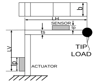
The schematic diagram of the proposed structure (i.e. inverted L) is shown in the Fig 1. This structure can be assumed to be made by joining two beams perpendicular to each other. The structure is mounted with two piezoelectric patches bonded on its surface acting as sensors and actuators. One of which are used as actuator and the other one as a sensor. The geometrical and mechanical properties of the structure are listed in table I. The Lagrange’s equations of motion for linear systems are given as below
( )
( )
( )
m t c k t
n ji i ji i ji i
t i,j 1,2,...,n
i 1 j
⎡ Δ + Δ + Δ ⎤
⎢ ⎥
⎣ ⎦
∑
= =
=
Q
(1)where Δ(t), Δ. (t) and (t)Δ.. are the physical displacement, velocity and acceleration respectively. Fig 1 shows the geometry and boundary conditions of the structural system. By using finite element techniques, the infinitely many-degree-of –freedom distributed system is approximated by an n-degree of freedom system in the form of global mass, damping and stiffness matrices The damping ratios are obtained by modal analysis. The eigenvalue problem can be solved to give the natural frequencies and mode shapes for various tip loads ranging from 0g – 20g. These modal parameters can be used to construct the system matrices [9, 10].
b
tp
ts
lp ACTUATOR
SENSOR
TIP LOAD LH
LV
Fig1: Schematic diagram of the inverted L structure
[image:2.595.348.500.64.197.2]B. Piezoelectric Sensing and Actuation
Table I: Geometrical and mechanical properties of the structure
When bending moment is given to the structure mounted with PZT patch, certain electrical charge is developed in it. Certain voltage is developed by this charge. This developed voltage is a function of the strain developed in the flexible structure on which this PZT patch is attached. This developed voltage is used as sensor response. On the other hand if a voltage V is applied to a patch attached on a distributed structure, a bending moment is produced [12]. This bending moment is used to reduce the vibrations.
III. ADAPTIVE FEEDBACK CONTROLLERS
Adaptive controller consists of two parts: a plant estimator and a controller parameter modifier. A plant estimator is receiving both the actuating signal and system output. The plant estimator estimates the system
Material
Property Steel PZT
Length of Horizontal limb(mm) LH= 100 ---
Length of Vertical Limb(mm) LV=100 ---
Thickness(mm) ts=1 tp=1
Length(mm) --- lp=20
Width(mm) B=10 b=10
Young’s Modulus(Mpa) Es=210 Ep=64
Density(Kg/m3) ρ
s =7800 ρp=5670
Distance of sensor from Free end i.e . x (mm)
60
Distance of actuator from Fixed end i.e. y (mm)
20
Distance of primary source of disturbance from jointed point i.e
. z (mm)
parameters. These parameters are fed to the controller parameter modifier.
A. Adaptive Minimum Variance Control
Adaptive Minimum Variance Controller (AMVC) uses directly the system parameters (i.e.
α s and β s in the difference equation form) and the controller parameters and the control input at instant of time t is given by
-β2(t)u(t-1)-β3(t)u(t-2)-....-βn (t)u(t-{n -1})b b
-α1(t)y(t)-α2(t)y(t-1)-...-αn (t)y(t-{n -1})a a
u(t)=
β1(t) (2)
B. Adaptive Pole Placement Control
In transfer function form, the structural system can be represented as a ratio of two polynomials G=B/A. An output feedback is
applied to the system which has a transfer function given by H=G/F. The overall transfer
function of the system is given by
1
= = =
+ +
P G BF
T
Q GH AF BG (3)
Which has CL zeros in P and CL poles in Q. The
co-efficient of the polynomial equation Q are
called the coefficients of CL characteristic equation. Since a s and b s are not available but their estimate is available i.e. α s and β s. This type of controller in which controller parameters are based on the CL poles is called Adaptive Pole Placement Controller (APPC).
C. Adaptive Linear Quadratic Control
In self tuning linear quadratic control, the controller parameters are updated, hence is called Adaptive Linear Quadratic Controller (ALQC). In this method, controller is chosen to minimize the steady state (t0 → -∞) cost function given as [14]
J=E {Q1 e2 (t) +R1 u2 (t)} (4)
where Q1 and R1 are the output and input weight age coefficients. To realize the above controller, spectral factors need to be calculated [15]. The optimal controller H=G/F can be calculated by
solving the coupled Diophantine equations, in terms of unknown polynomials G and F.
IV IMPLEMENTATION AND VERIFICATION OF CONTROL SYSTEMS
A. Experimental Setup and Procedure
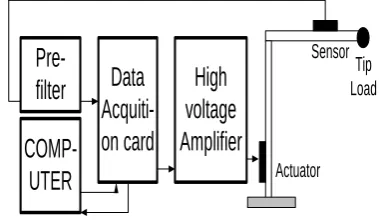
The schematic view of the inverted L structure along with the hardware is shown in the fig 2. The inverted L structure is equipped with 2 PZT patches. One of these is being used as sensor and the other as actuators. The strain developed due to vibrations is converted into electrical voltages, and is measured at the output sensor or error sensor. The observed signal is in the range –10 volt to +10 volt. This does not need amplification. To remove the effect of higher modes the signals are pre – filtered. Then the signal goes to data acquition card. Analog-to-digital (A/D) conversion of the signal is done in this card. To bear the computational burden LABVIEW based real time engine 8187 RT is used.
COMP-UTER
Data
Acquiti-on card
High
voltage
Amplifier
Actuator Sensor
Pre-filter
[image:3.595.339.530.396.506.2]Tip Load
Fig 2 Schematic diagram of the experimental setup
Based on these digitized, input signals, control signals are calculated by the real time engine. These signals are in the range of –10 V to +10V. After digital-to-analog (D/A) conversion in the data acquition card, control signal goes to the high voltage amplifier MA-17 manufactured by APEX Technologies.
B. Simulation and Experimental Results
ensured and hence applied in the present work. In the dead zone, parameter adaptation stops and hence the parameters are not updated. Standard methods of system parameters adaptation can be
combined with dead zone approach.
Same parameter (i.e. system) identification techniques are applied to all the controllers. The system corresponding to zero gram tip load is
taken as nominal system. The tip load is changed
from 0g to 5g and 0g to 15g. Maximum available actuator voltage is taken as 220 volt.
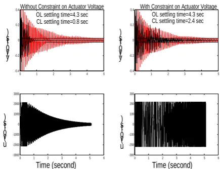
In the present study, first two modes are controlled simultaneously. In these situations, AMVC requires very high amplitude of actuator voltages. If 220 volts is put as a constraint on the magnitude of actuator voltage, the actuator voltage does not decrease as the amplitude of vibration decreases. This makes the CL system to be noise sensitive. A settling time of 2.4 second is obtained for the nominal system if no constraint on the peak actuator voltage is applied (fig 3). As the tip load changes to 5g, the MVC becomes unstable. By using the AMVC, a settling time of 0.8 second is achieved if actuator voltage of magnitude 2500 volts is available. Similar results were found for large changes in system parameters. Constant decrease in the amplitude of actuator voltage is obtained in that case (fig 3c). Since, such high voltages are not normally available in real life situations; a magnitude constraint had to be applied on the actuator voltage. By applying the magnitude constraint on the peak actuator voltage, even at lower amplitudes, actuator voltage does not decrease (fig 3d). This is not desirable due to the reason mentioned above. By observing the peak actuator voltage graph (fig 3) minutely, it is quite obvious that there is abrupt change of sign of the actuator voltage. This reduces the life of piezoceramics based actuators and hence objectionable.
Establishing this fact, Spearritt et al [17] concluded that the PVDF film actuators can easily be destroyed due to abrupt change of control voltage. The life of the PZT actuators also decreases due to this problem. Ashokanathan et al. [18] solved this problem up to some extent by using modified Lyapunov control law instead of ordinary Lyapunov control law used by Spearritt. In this method the voltage which changes
abruptly in sign was replaced by continuous – time voltage. Based on these considerations, it is obvious that, AMVC should be avoided for multi-modal vibration suppression.
0 1 2 3 4 5
-0.4 -0.2 0 0.2 0.4
Time (second) y
(v olt s )
Without Constraint on Actuator Voltage
0 1 2 3 4 5
-0.4 -0.2 0 0.2 0.4
Time (second) y(v
olt s)
With Constraint on Actuator Voltage
0 1 2 3 4 5 6
-3000 -2000 -1000 0 1000 2000 3000
u(v olt s)
0 1 2 3 4 5 6
-300 -200 -100 0 100 200 300
u(v olt s)
OL settling time=4.3 sec CL settling time=0.8 sec
[image:4.595.337.555.123.290.2]OL settling time=4.3 sec CL settling time=2.4 sec
Fig 3: Effect of actuator voltage amplitude on system performance with AMVC
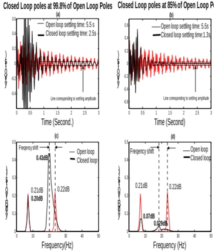
In case of APPC, the CL settling time of the nominal system is 2.2 second. The corresponding OL settling time is 4.5 second. If PPC is applied, the CL settling time of the nominal system is 1.35 second. So, it can be safely concluded that even by using the adaptive version of PPC, the performance deterioration is resulted for the nominal system. But there is not complete deterioration as the CL settling time (2.2 second) is quite less than OL settling time (4.5 second). On the contrary, in single mode control, there is complete deterioration in the performance, in which the OL and CL settling times are the same. So, application of APPC in its direct form is not desirable. By changing the position of CL poles, this problem can be avoided. As the CL poles were changed from 99.8% to 85% of OL poles (in imaginary part only), better over all performance was observed. Fig 4 shows the performance of APPC with different positions of CL poles. With new position of CL poles, no performance deterioration is resulted for the nominal system (Fig 4b).
volt. Fig 5 shows the performance comparison of different control strategies when tip load changes from zero to 5 gram. Obviously, using ALQC, less control effort was required than with APPC (Fig 5 b &d).
In case of large changes in system parameters (0g-15g), fixed PPC becomes unstable. APPC also gives poor performance (Fig 6 a & c) if applied in its direct form (i.e. giving no consideration to CL pole positions). The second mode is excited instead of being suppressed. By shifting the CL poles in APPC (with CL poles as 85% of OL poles in imaginary part only), better performance gets resulted. The CL settling time of
1.3 second instead of 2.5 second is obtained. The
second mode was suppressed considerably (Fig 6 b & d). So, if large variations in system parameters are expected, APPC (with optimal
position of CL poles) is quite efficient. One thing
worth observing in table 5 is that, by using APPC, the settling time of the CL system remained nearly fixed (1.0-1.3 second) in spite of large changes in system parameters (i.e. 0g-15g).
0 0.5 1 1.5 2
-0.5 0 0.5 y (V olt s )
CL poles at 99.8% of OL Poles
0 0.5 1 1.5 2
-150 -100 -50 0 50 100 150 u(V olt s)
0 0.5 1 1.5 2
-0.5 0 0.5 y(V olt s) Time (Second)
0 0.5 1 1.5 2
-150 -100 -50 0 50 100 150 Time (Second) u(V olt s )
CL poles at 85% of OL Poles
(a) (b)
(c) (d)
OL response CL response
[image:5.595.329.531.49.223.2]OL response CL response
Fig 4: Effect of pole locations on nominal system performance at zero tip load
By using the adaptive version of LQC for a tip load of zero grams, a CL settling time of 1.3 second is obtained as compared with LQC with CL settling time of 1.0 second (table II). So, even by using the ALQC, the performance degradation of the nominal plant still exists.
0 1 2 3 4 5 6 -1 -0.5 0 0.5 1 APPC Time(Second) y(V olt )
0 1 2 3 4 5 6 -1000 -500 0 500 Time(Second) u(V olt )
0 1 2 3 4 5 6 -1 -0.5 0 0.5 1 ALQC Time(Second) y(V olt )
0 1 2 3 4 5 6 -400 -200 0 200 400 Time(Second) u(V olt )
2.1s 4.3s 2.0s 4.3s
OL response CL response
[image:5.595.63.271.399.578.2]OL response CL response
Fig 5: Time domain performance comparison of different control strategies when tip load changes
from 0g to 5g
Next, for small changes in system parameters (0-5g), a CL settling time is 2.0 second. The corresponding settling time for LQC is 2.2 second i.e. by applying ALQC performance degradation even at small
changes in system parameters is not there.
This is contrary to APPC in which significant performance degradation near the nominal plant is always there, if no consideration was given to the position of CL poles. At large changes in system parameters (0-15g), a CL settling time of 3.2 second is obtained. So for small as well as large changes in system parameters, ALQC gives consistently better performance.
0 0.5 1 1.5 2 2.5 3 -0.4 -0.2 0 0.2 0.4 0.6 y(V olt s) Time (Second.)
0 10 20 30 40 50
0 0.1 0.2 0.3 0.4 0.5 y(d B(v olt s)) Frequency (Hz)
0 0.5 1 1.5 2 2.5 3 -0.6 -0.4 -0.2 0 0.2 0.4 0.6 y (V olt s ) Time (Second)
0 10 20 30 40 50
0 0.1 0.2 0.3 0.4 0.5 y(d B(v olt s)) Frequency(Hz)
Open loop settling time: 5.5s Closed loop settling time:1.3s Open loop settling time: 5.5 s
Closed loop settling time: 2.5s
Open loop Closed loop
Open loop Closed loop
(a) (b)
(c) (d)
Line corresponding to settling amplitude Line corresponding to settling amplitude Closed Loop poles at 99.8% of Open Loop Poles Closed Loop poles at 85% of Open Loop Poles
0.21dB
0.20dB
0.22dB
0.43dB Freqency shift
Freqency shift
0.21dB 0.22dB
0.07dB 0.029dB
[image:5.595.340.554.489.741.2]The experimental OL settling time of 4.6 second was obtained. This differs from theoretical OL settling time of 4.9 second. First of all, AMVC was applied. The initial controller was designed according to nominal system corresponding to 0g tip load. The adaptation of controller parameters was started from these initial parameters. A CL settling time of 2.0 second was obtained. The peak control voltage was continuously forced to decrease from 220 volts. After that APPC was tested. The CL system with controller gains corresponding to 85% value (i.e. CL poles were 85% of OL poles in terms of imaginary part) becomes unstable in the presence of noise. This is probable due to high value of
controller gains. Theoretically, the CL system
remains stable for these controller gains. To maintain stability, this value was increased to 92
%. The controller gains with this value are
acceptable experimentally. The CL settling time
of 2.0 second was obtained. Almost similar performance was obtained using the ALQC. The maximum allowable actuator voltage was limited to 220 volts. To obtain the similar performance the control effort required in APPC is 7-16 times higher in that in ALQC. The control effort was calculated by using the relation,
Settling Time 2 0
control effort=
∫
u (t) x sampling interval. This high value of control effort is wasted in exciting the inverted L structure at 20 Hz for certain period of time. Since online spectral factorization is computational intensive, ALQC can not be implemented on computers running with windows based operating system. A LABVIEW based real time engine 8187RT was used to implement ALQC. This real time engine is provided by NATIONAL INSTRUMENTS and works on real time operating system.V. CONCLUSION
Stability problem is quite intensive in case of multiple mode vibrations. In adaptive minimum variance control, although the computational burden is small, there is a sudden change in the sign of actuator voltage. This aspect reduces the life of actuators. In adaptive pole placement control, the computational burden is manageable, but excitation of the structure to certain other frequencies different from modal frequencies is
there. This aspect increases the control effort requirements to a very high value. Adaptive linear quadratic control is free from all these limitations. Real time engines working on real time operating systems can bear high computational burden. Study can be extended to MIMO systems easily.
REFERENCES
[1]. Tzes A P and Yurkowich S “Application and comparison of on-line identification methods for flexible manipulator control” International journal of robotic research10(5), 1991 pp. 515-527
[2]. Zeng Y, Araujo and Singh SN “Output feedback variable structure adaptive control of a flexible spacecraft”
Astronautica44(1), 1999, pp 11-22
[3]. Youn SH, Han JH and Lee I “Neuro-adaptive vibration control of composite beams subjected to sudden de-lamination” Journal of sound and vibration 238(2),
2000, pp. 215-231
[4]. Shaw J “Adaptive control for sound and vibration: A comparative study ” Journal of sound and vibration
235(4), 2000, pp. 671-684
[5]. Rew KH “Multi-modal vibration control using adaptive positive position feedback” Journal of intelligent materials and structures13 (1), 2002, pp. 13-22
[6]. Bai MR “Experimental evaluation of adaptive predictive control for rotor vibration suppression” IEEE transactions on control system technology 10(6), 2002,
pp. 895-901
[7]. Lim CW, Chung TY and Moon SJ “Adaptive bang-bang control for the vibration control of structures under earthquakes” Earthquake Engineering and Structural Dynamics32(13), 2003, pp. 1977-1994
[8]. Xiongzhu Bu, Lin Ye, Zhongqing Su and Chunhui Wang “Active control of flexible smart beam using system identification technique based on ARMAX”, Journal of Smart Materials and Structures12, 2003, pp. 845-850.
[9]. Meirovitch, “Elements of Vibration Analysis” McGraw
Hill Publishing Company, New York, 1986
[10]. Meirovitch, “ Dynamics and Control of Structures”
John Wiley and sons UK, 1986
[11]. Buttler R and Vittal Rao “A State Space Modeling and Control Method for multivariable smart structural Systems” Smart Materials and Structures 5, 1996, pp.
386-399
[12]. Baz A, and Poh S, “Performance of Active Control System with piezoelectric actuators” Journal of Sound and Vibration 126(2), 1988, pp. 327-343
[13]. Wellstead PE, D Prager and P Zanker “Pole Assignment self tuning regulator” Proc. IEE Control Science126,
1981, pp. 781-87.
[14]. Grimble MJ “Implicit and explicit LQG self-tuning controllers” Automatica 20(5), 1984, pp. 661-669
[15]. Shaked U “A general transfer function approach to linear stationery filtering and steady state optimal control problems” Int. Journal of Control24, 1976, pp. 741-770
[16]. Spearritt DJ and Ashokanathan SF “Torsional Vibration Control of a Flexible using Laminated PVDF Actuators”
Journal of Sound and Vibration, 193(5), 1996, pp.
941-956
[17]. Ashokanathan SF and Gu M, “Torsional vibration control of flexible rod using laminated PVDF actuators”