C++ version of the algorithm.

Abstract

—

to existing software versions.

Index Terms—Hardware Design, High Performance

Computing, Iterative Methods, Parallelization.

I. INTRODUCTION

A huge number of physical, chemical, and biological phenomena are described by means of Partial Differential Equations (PDEs). Examples of such phenomena are the motion of fluids [1], energy dissipation, Belousov-Zhabotinsky reactions, and DNA matching. In addition, different applications in finance and economics [2], computer vision [3],[4], computer graphics [5], image processing [6-7], weather simulation [8], statistical physics [9], and computational physics [10] can be modeled using PDEs. Understanding, analyzing and solving these equations, efficiently, allows us to find the answers to the modeled systems or applications [11]. For this reason, a number of algorithms have been devised for solving PDEs with increasing precision.

Research has proved that the most powerful solver is the Multigrid algorithm [12-13]; which combines classical iterative algorithms, such as Gauss-Seidel, with subgrid refinement steps to give a method superior -in terms of

Manuscript received March , 2007.

Safaa J. Kasbah is with the Division of Computer Science and Mathematics, Lebanese American University, Beirut, Lebanon (phone: 961-3-788402; email: [email protected]).

Issam W. Damaj is with the Department of Electrical and Computer Engineer, Dhofar University, Salalah, Sultanate of Oman (e-mail: [email protected]).

storage and computation-to classical iterative techniques. However, the computation of MG becomes complex and time consuming [7] as the complexity of the system or phenomena, to be modeled, increases.

Many attempts for exploiting the inherent parallelism of Multigrid have been made to achieve the desired efficiency and scalability of the method [14-15]. Yet, most efforts fail in this respect due to many factors (time and resources) governed by software implementations.

In the last decade, a new computing paradigm, Reconfigurable Computing (RC), has emerged. RC-systems overcome the limitations of the two well known computing paradigms: 1) General Purpose Processors (GPPs) in the form of software and 2) Application Specific Integrated Circuits (ASICs) in the form of hardware. RC-systems combine the flexibility offered by software and the performance offered by hardware [16-18]. It requires a reconfigurable hardware, such as an FPGA, and a software design environment that aids in the creation of configurations for the reconfigurable hardware [16]. RC -systems have successfully accelerated a wide variety of applications. Most of these applications have been reported in the fields of: signal processing (e.g. weather forecasting, seismic data processing, Magnetic Resonance Imaging (MRI), adaptive filters), cryptography and DNA matching.

In this paper, we present a hardware implementation of the V-cycle MG algorithm for the solution of a 2D-Poisson equation using different classes of FPGAs: Xilinx Virtex II Pro, Altera Stratix and Spartan3L which is embedded on the RC10 board from Celoxica. We use Handel-C, a higher-level design tool, to code our design which is analyzed, synthesized, and placed and routed using the FPGAs proprietary software (DK Design Suite, Xilinx ISE 8.1i and Quartus II 5.1). We compare our implementation results with existing software version of the algorithm, since there are no hardware implementations of MG in the literature. A general overview of Multigrid solvers in general, and the V-cycle MG solver in particular is presented in Section 2. In Section 3, we describe our proposed hardware implementation of the V-cycle MG for the solution of 2D -Poisson equation. Then, the implementation results are presented in Section 4. Our results are compared with available software version results, written in C++ and running on a general purpose processor. Section 5 concludes the work and presents possible future directions.

High-Performance Multigrid Solvers in

Reconfigurable Hardware

Safaa J. Kasbah and Issam W. Damaj

II. MULTIGRID SOLVERS: AN OVERVIEW

Multigrid methods are fast linear iterative solvers used for finding the optimal solution of a particular class of partial deferential equations. Similar to classical iterative methods (Jacobi, Successive Over Relaxation (SOR) and Gauss Seidel), an MG method starts with an approximate solution to the differential equation; and in each iteration, the difference between the approximate solution and the exact solution is made smaller [19].

In general, the error resulting from the exact and approximate solution will have components of different wavelengths: high-frequency components and low-frequency components [22]. Classical iterative methods reduce high-frequency/oscillatory components of error rapidly, but reduce low-frequency/smooth components of error much more slowly [21].

The Multigrid strategy overcomes the weakness of classical iterative solvers by observing that components that appear smooth on fine grid may appear oscillatory when sampled on coarser grid [22]. The high-frequency components of the error are reduced by applying any of the classical iterative methods. The low-frequency components of error are reduced by a coarse-grid correction procedure [19-20].

A typical Multigrid cycle starts by applying any classical iterative method (Jacobi, Gauss Seidel or Successive Over Relaxation) to find an approximate solution for the system. The Residual operator is then applied to find the difference between the actual solution and the approximate solution. The result of this operator measures the goodness of the approximation. Since it is easier to solve a problem with less number of unknowns [13],[21]; a special operator-Restriction- for mapping the residual to a coarser grid (less number of unknowns) - is applied for several iterations until the scheme reaches the bottom of the grid hierarchy. Then, the coarse grid solver operator is applied to find the error on the coarsest grid. Afterwards, the interpolation operator is applied to map the coarse grid correction to the next finer grid in an attempt to improve the approximate solution. This procedure is applied until the top grid level is reached giving a solution with residual zero. Finishing with several iterations back to the finest grid gives a so-called- V-cycle Multigrid [12]. The MG algorithm is summarized in Fig. 1; the Multigrid basic operators are depicted in Fig. 2.

Fig. 1: Multigrid Algorithm

Fig. 2: V-cycle Multigrid

In this work, the V-cycle MG method is used to find the solution to a 2D-Poisson equation in the form:

y x

f y x u y y x u

x 2 ,

2

2 2

) , ( )

,

( =

∂ ∂ + ∂

∂ ₍₁₎

III. HARDWARE IMPLEMENTATION OF V-CYCLE

MULTIGRID

All available Multigrid solvers are realized as software running on general purpose processors [20-21]. Available software packages have been implemented in C, Fortran-77, Java and other languages, where parallelized versions of these packages require inter-processor communication standards such as Message Passing Interface (MPI) [18]. Each of these packages attempt to achieve an efficient and a scalable version of the algorithm by compromising between the accuracy of the solution and the speed of realizing the solution.

The V-cycle Multigrid algorithm has been designed and implemented using Handel-C, a higher-level hardware design tool. Our choice was based on the language’s features for rapid and efficient prototyping; since Handel-C syntax is similar to the ANSI-C with additional extensions for expressing parallelism. The Handel-C compiler comes packaged with the Celoxica DK Design Suite [25].

Our design has been tested using the Handel-C simulator; afterwards, we have targeted a Xilinx Virtex II Pro FPGA, an Altera Stratix FPGA, and an RC10 board from Celoxica. The tools provided by the device’s vendors were used to synthesize and place & route the design[25-27]

The Multigrid method can be parallelized by parallelizing each of its components; i.e., smoother, coarse grid solver, restriction and prolongation. Each of these components is parallelized by using the Handel-C construct ‘par’. This is used whenever it was possible to execute more than one instruction in parallel without affecting the logic of the source code. The results obtained show a substantial improvement in the MG performance when compared to a traditional way of executing instructions on a GPP, as depicted in the following Fig. 3 and Fig. 4 for the two MG operators Restrict Residual and Correct.

Finding the solution to PDEs using MG requires floating point arithmetic operations which are 1) far more complex, and 2) consume more area than fixed point operations. For this reason, Handel-C does not support floating point type. Yet, floating point arithmetic can be performed using the Pipelined Floating Point Library provided in the Platform Developer’s Kit.

Unfortunately, a failure in the Handel-C simulator persists whenever the number of floating point arithmetic operations exceeds four. We were notified that a fixed 1. Perform few pre-smoothing Gauss-Seidel (or any

iterative method) iterations to reduce the short wavelength errors in the solution.

2. Compute Residual

3. Restrict Residual (fine Æ coarse) 4. Solve residual equation

5 Interpolate solution(coarse Æ fine) 6. Update the solution

7. Perform few post-smoothing Gauss-Seidel (or any iterative method) iterations and return the improved solution to the next finer grid.

S: Smooth R: Restrict P: Prolongate

Solve on coarsest grid

P R

version of the DK simulator will be available in a future release of DK. The only possible way to avoid the simulator’s failure, in the current version, was to convert/Unpack the floating point numbers to integers and perform integer arithmetic on the obtained unpacked numbers, as shown in Fig. 3, 4 and 5. Though it costs more logic to be generated, the integer operations on the unpacked floating point numbers have a minor effect on the total number of the design’s clock cycles.

Originally, the Multigrid method depends on recursion, which cannot be supported by Handel-C. An iterative version of the algorithm is designed and shown in Fig. 6. Only a snapshot of the parallel version of (Smoother, Find Residual, Prolongate) MG components is shown in the figure. Their implementation style is very similar to what is shown in Fig. (3d) and Fig. (5a). Details about Restriction and Correct operators are shown in Fig. 3, Fig. 4, and Fig. 5.

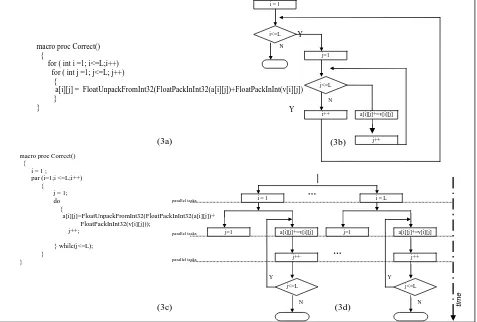
Fig. 3: Correct operator, illustrating the effect of using par construct: (3a), (3b), (3c) and (3d) shows sequential code, flow charts, parallel code and combined flow chart/concurrent process model, respectively. The dots represent replicated instances in d).

macro proc Correct() {

for ( int i =1; i<=L;i++) for ( int j =1; j<=L; j++) {

a[i][j] = FloatUnpackFromInt32(FloatPackInInt32(a[i][j])+FloatPackInInt(v[i][j]) }

}

macro proc Correct() {

i = 1 ; par (i=1;i <=L;i++) {

j = 1;

do

{

a[i][j]=FloatUnpackFromInt32(FloatPackInInt32(a[i][j])+ FloatPackInInt32(v[i][j]));

j++;

} while(j<=L); }

}

Y

N _time

parallel tasks

parallel tasks

a[i][j]+=v[i][j]

j++

i = 1 i = L

j=1

j<=L

Y

N a[i][j]+=v[i][j]

j++ j=1

j<=L

parallel tasks

(3d) (3a)

(3c)

a[i][j]+=v[i][j]

Y

N

Y

N

j<=L i = 1

j++ i++

j=1 i<=L

(3b)

macro proc Restrict_Residual() {

for (I=1;I <= L2;I++) {

i = 2 * I - 1;

addCycles = FloatPipeAddCycles;

for ( J=1;J<=L2;J++)

{

addCycles = FloatPipeAddCycles;

j = 2 * J - 1;

op1 = FloatUnpackFromInt32(FloatPackInInt32(r[i][j]) + FloatPackInInt32(r[i+1][j]));

op2 = FloatUnpackFromInt32(FloatPackInInt32(r[i][j+1]) +FloatPackInInt32(r[i+1][j+1]));

opResult = FloatUnpackFromInt32(FloatPackInInt32(op1) + FloatPackInInt32(op2));

I<=L2 I = 1

i = 2 * I - 1

addCycles=FPipeAddCycl

J=1

j<=L2

N

I++

Y

addCycles=FPipeAdd

i = 2 * J-1

op1=r[i][j]+r[i+1][j]

op2=r[i][j+1]+r[i+1][j+1]

opResult = op1 + op2

R[i][j]=fFactor*opREsult

J++ (4b)

(4a)

Fig. 4:Restrict Residual operator sequential version: (4a), (4b) shows sequential code and the flow chart.

Fig. 5: Restrict Residual operator, illustrating the effect of using par construct: (5a) and (5b) shows parallel code and combined flow chart/concurrent process model, respectively. The dots represent replicated instances

Fig. 6:V-cycle MG, iterative version version each component parallelization. The dots in each of the component’ combined flowchart/concurrent process model represent replicated instances.

START N I=1 I=L N Y J=2*J-1 v[i][j]=V[I][J] v[i+1][j]=V[I][J] v[i][j+1]=V[I][J] v[i+1][j+1]=V[I][J] J++ J<=L2 N Y J=2*J-1 v[i][j]=V[I][J] v[i+1][j]=V[I][J] v[i][j+1]=V[I][J] v[i+1][j+1]=V[I][J] J++ J<=L2 N Y I=1 i=2*I-1 I=2 J<=L v[I][J]={0,0,0} J++

I=0 I=2 I=L2

Y J<=L v[I][J]={0,0,0} J++ N I=1 i=2*I-1

...

...

...

...

i=1 i=2 i=L

j=1 j=L j<=L op2=psiNew[i][j-1] + psiNew[i][j+1] op1=psiNew[i-1][j] + psiNew[i+1][j] addCycles= FloatPipeAddCycles sq_h=my_h*my_h opResult=op1+op2 temp1=sq_h*rho[i][j] addCycles!=0 addCycles--psiNew[i][j]=tmp2*fFactor tmp2=opResult+tmp2 j++ Y N Y N j<=L op2=psiNew[i][j-1] + psiNew[i][j+1] op2=psiNew[i-1][j] + psiNew[i+1][j] addCycles= FloatPipeAddCycles sq_h=my_h*my_h opResult=op1+op2 temp1=sq_h*rho[i][j] addCycles!=0 addCycles--psiNew[i][j]=tmp2*fFactor tmp2=opResult+tmp2 j++ i=1 j=1

...

...

G auss_S eidel Y

N

Initialize

Solve on Coarse Grid Pre-Smoothing

Correct

Post-Smoothing Prolongate

Finest level?

Find Residual Restrict Residual STOP Y Y N Y N Y N N

i=0 i=2 i=L

op1 = {0,0,0} op2 = {0,0,0} op3 = {0,0,0} opResult={0,0,0} fResult = {0,0,0}

j=0 j++ r[i][j]=rho[i]j] j<=L Y j=0 j++ r[i][j]=rho[i]j] j<=L I=1 j=1 I=2 I=L op1=psiNew[i+1][j] + psiNew[i-1][j] op2=psiNew[i][j+1] + psiNew[i][j-1] addCycles= FloatPipeAddCycles sq_h=my_h*my_h tmp1=psiNew[i][j]*4

op3 = op1+op2

addCycles!=0 addCycles--temp2=sq_h+sq_h opResult=op3-tmp2 r[i][j]=r[i][j]+opResult j++ j<=L

...

...

...

par (I=1;I <= L2;I++) {

par{ i = 2 * I - 1;

addCycles = FloatPipeAddCycles; J = 1;

} do { par {

addCycles = FloatPipeAddCycles; j = 2 * J - 1;

} par {

op1=FloatUnpackFromInt32(FloatPackInInt32(r[i][j])+FloatPackInInt32(r[i+1][j])); op2=FloatUnpackFromInt32(FloatPackIn32(r[i][j+1])+FloatPackInt32(r[i+1][j+1])); opResult = FloatUnpackFromInt32(FloatPackInInt32(op1)+FloatPackInInt32(op2)); R[I][J]=FloatUnpackFromInt32(FloatPackInt32(fFactor)*FloatPackInt32(opResult));

J++;

} } while (J<=L2); Y

J++ R[i][j]=fFactor*opREsult

opResult = op1 + op2

op2=r[i][j+1]+r[i+1][j+1] op1=r[i][j]+r[i+1][j]

i = 2 * J-1 addCycles=FPipeAdd

I = 1

addCycles=FPipeAdd J=1

j<=L2

I =2

i = 2 * I - 1

I =L

(5a) (5b)

IV. EXPERIMENTAL RESULTS

The Handel-C simulators along with the FPGA vendor’s tools were used to obtain the results. We draw a comparison of the execution time between our results and a software version written in C++, compiled using Microsoft Visual Studio .Net (2003) [21], and running on a Pentium (M) processor 2.0 GHz, 1.99 GB of RAM. The obtained results are based on the following criteria:

• Speed of convergence: the time it takes the Multigrid method to find the solution to the PDE in hand. The speed of convergence is measured using the clock cycles of the design –using the simulator-divided by the frequency at which the design operates at-using the generated timing analysis report.

• Accuracy of the solution: The convergence of the Multigrid algorithm is greatly dependent on the accuracy of the solution. The increase in the accuracy results in the increase in both the computation and the logic utilization. In this work, the required solution is realized as soon as an adequate degree of accuracy is obtained [21]. • Chip-area: this performance criterion measures

the number of occupied slices on the FPGA on which the design is implemented. The number of occupied slices is generated using the FPGA vendor’s place and route tool.

The following selections were used for all tests. • Restriction: Full Weighting

• Interpolation: Bilinear

• Number of smoothing steps: v1=v2=2

(v1_aPresmoothing,v2_aPostsmoothing)

• Smoother used: Gauss-Seidel

• Accuracy: 0.001 for all Handel-C test cases and C++ test cases up to problem size 64x64.

The timing results for Virtex II Pro FPGA (2vp7ff672-7) are shown in Table 1. We report the execution time for different problem sizes, along with the maximum frequency at which each design operates at. Execution time is calculated using: No. of clock cycles/Max. Frequency.

Table 1:Execution Time + Max frequency for different problem sizes

Mesh Size Execution Time(ms) Fmax(MHz)

8x8 0.000063 159.74 16x16 0.00026 153.52 32x32 0.00118 136.15 64x64 0.00555 115.97

128x128 0.031 83.91

256x256 0.188 54.60

512x512 1.308 31.45

1024x1024 9.3 17.60

2048x2048 70.97 9.28

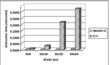
Fig.s 6 and 7 show the results of comparing the execution time when running a C++ version of the V-cycle Multigrid

algorithm and our proposed Handel-C version. The superiority of the hardware implementation over the software implementation is clear in both figures. However, for a problem size greater than (64x64), it becomes difficult to measure the execution time of the software (C++) version with the same accuracy of 0.001. At that time, our concern was to force the C++ version of MG to converge at any price. This was only possible by sacrificing with the accuracy of the solution; where we had to gradually increase this factor until we reached an accuracy of 2.0 for a problem size of 2048x2048, in contrast to an accuracy of 0.001 for a problem size of 8x8. On the other hand, Handel-C results were independent from the accuracy of the solution. The accuracy was constant all the way from a problem size of 8x8 to 2048x2048. Obviously, this explains the degeneration of the speedup indicated in Fig. 7.

0.0005 0.0505 0.1005 0.1505 0.2005 0.2505 0.3005

E

x

e

c

ut

io

n

t

ime

(

s

e

c

on

ds

)

8x8 16x16 32x32 64x64

M esh size

Handel-C

C++

Fig. 7:Execution time of Handel-C implementation vs. C++ implementation lower side results.

0 10 20 30 40 50 60 70 80 90

E

x

e

c

ut

ion t

im

e

(

s

e

c

ond

s

)

128x 128

256x 256

512x 512

1024 x102

4

2048 x204

8

Mesh size

Handel-C C++

Fig. 8: Execution time of Handel-C implementation vs. C++ implementation upper side results.

In Table 2 we draw a comparison between the accuracy of the solution for each of the C++ and Handel-C test cases. The speedup of the design is calculated as the ratio of Execution Time (C++) / Execution Time (Handel-C). Tables 3, 4 and 5 show, respectively, the Virtex II Pro (2vp7ff672-7), Spartan3L (3s1500lfg320-4) and Altera Stratix(EP1S10F484C5) FPGA synthesis results for different problem sizes. When targeting Xilinx Virtex II Pro FPGA, the largest possible problem size that we could achieve was 2048x2048, where 99% of the slices were utilized. Meanwhile, the largest possible problem size was 512x512 when targeting the Spartan3LFPGA.

Table 2: Required accuracy of the solution for C++ and Handel-C test cases, and the design speedup

Table 3:Virtex II Pro Synthesis results using Xilinx ISE

Mesh Size Number of

Occupied Slices

Total equivalent gate count

8x8 264(5%) 5,990

16x16 295(5%) 6,497

32x32 415(8%) 9,321

64x64 536(8%) 12,376

128x128 789(16%) 18,107

256x256 1,247(25%) 29,244

512x512 2,125(43%) 51,115 1024x1024 3,875(43%) 94,484

2048x2048 4,926(99%) 180,879

Table 4:Spartan3L Synthesis Results using Xilinx ISE

Mesh Size Number of

Occupied Slices

Total equivalent gate count

8x8 687(20%) 355,687

16x16 717(21.5%) 356,163

32x32 769(23%) 357,224

64x64 832(25%) 358,921

128x128 1049(32%) 361,956

256x256 1507(45.3%) 367,673

512x512 3187(96%) 375,293

Table 5:Altera Stratix synthesis results using Quartus II

Mesh Size

Total Logic Elements

Logic element Usage by Number of LUT Inputs

Total Registers

8x8 725 402 228

16x16 818 554 265

32x32 925 625 301

64x64 1068 709 360

128x128 1307 841 467

256x256 1739 1,070 670

512x512 2653 1,357 816

1024x1024 3491 1,809 1002

2048x2048 4501 2,201 1482

The above experimental results demonstrate that implementing the MG algorithm on hardware outperforms a software version of the algorithm.

V. CONCLUSION AND FUTURE WORK

In this paper, we have presented a hardware implementation of the V-cycle Multigrid method for solving the Poisson equation in two dimensions. Handel-C hardware compiler is used to code and implement our design and map them onto high-performance FPGAs, such as, Virtex II Pro, Altera Stratix, and Spartan3L which is embedded in the RC10 FPGA-based system from Celoxica. The implementation performance is analyzed using the FPGAs vendors’ proprietary software. Moreover, we compare our implementation results with available software version results running on General Purpose Processors and written in C++. The obtained results have demonstrated that MG on hardware outperforms MG on GPP. A speedup of 142.86 was achieved for a problem size of 8x8, whereas a speedup of 1.14 was achieved for 2048x2048. This degeneration of the speedup is due to the increase of the value of the required accuracy of the solution.

Possible future directions include realizing a pipelined version of the algorithm, moving to a lower-level HDL such as VHDL, mapping the algorithm into a coarse grain reconfigurable systems (e.g., MorphoSys) [28], and benefiting from the advantages of formal modeling [29]. We can also extend the benefit of MG in solving nonlinear partial differential equations by implementing the Algebraic Multigrid algorithm.

VI. REFERENCES

[1] N. Foster and R. Fedkiw, “Practical animation of liquids,” in

Proceedings of the 28th annual conference on Computer graphics and interactive techniques, 2001, pp. 23-30

[2] B. Aruoba and J. Fernandez-Villaverde, J. “Comparing Linear and

Nonlinear Solution Methods for Dynamic Equilibrium Economies,” Computing in Economics and Finance, Society for Computational

Economics. http://www.depts.washington.edu/sce2003/Papers/133.pdf.2003.

[3] M. Nielsen, P. Johansen, O. F. Olsen, and J. Weickert,editors, Scale

Space Theories in Computer Vision, in Lecture Notes in Computer Science, v. 1682, 1999, Springer-Verlag, Berlin.

[4] R. P. Fedkiw, G. Sapiro and C.W. Shu, “Shock Capturing, Level Sets

and PDE Based Methods in Computer Vision and Image processing: a review on Osher’s Contribution,” Journal of Computational Physics, vol. 185, no. 2, pp.309-341, 2003.

[5] R. Whitaker and D.T Chen, “Embedded active surface for volume

visualization,” SPIE Medical Imaging VIII, 2167, February 1994, pp. 340-352.

[6] L. Gorelick, M Galun, E. Sharon, R. Basri, and A. Brandt, “Shape

representation and classification using the poisson equation,” IEEE Conference on Computer Vision and Pattern Recognition (CVPR), Washington, DC, USA . vol. 3, pp. 61–67, 2004

[7] M. Arigovindan, M. Sühling, P. Hunziker, and M. Unser, “ Multigrid

image reconstruction from arbitrarily spaced samples,” International Conference on Image Processing, vol. 3, pp. 381-384, 2002.

[8] G. Longo, “ Computer Modelling and Natural Phenomena,” In ACM

SIGSOFT Software Engineering Notes. ACM Press, vol. 28, no. 5. pp. 1-5, 2003.

[9] D. Kandel, E. Domany, and A. Brandt, “Simulations without critical

slowing down: Ising and three-state Potts model,” Physical Review B. vol. 40, no. 1, 1989.

Mesh Size Accuracy Speedup

C++ Handel-C

8x8 0.001 0.001 142.86 16x16 0.001 0.001 185.59 32x32 0.001 0.001 119.23

64x64 0.001 0.001 58.56

128x128 0.2 0.001 20.77

256x256 1 0.001 5.25

512x512 1.1 0.001 2.92

1024x1024 1.3 0.001 1.58

2048x2048 2 0.001 1.14

[10] R. Brower, “Non-Abelian Projective Multigrid for Lattice Gauge Theory,” Physical Review Letters,vol. 66, no. 10, 1991.

[11] B. Diskin and V. Harik, “On Efficient Multigrid Methods for

Materials Processing Flows with Small Particles”. NASA NIA

report, 2004. http://www.nianet.org/technicalreports/pdfs/2004/2004-01.pdf.

[12] W. L. Briggs, V.E. Henson and S.F. Mccormick,. A Multigrid

tutorial, SIAM, Philadelphia, PA, second ed. 2000.

[13] A. Brandt, “Multi-Level Adaptive Solutions to Boundary Value

Problems,” Math. Comp, vol. l., no. 31, pp. 333-390, 1997.

[14] K. Nakajima, “Parallel Multilevel Iterative Linear Solvers for

Large-Scale Computations,” ACES 2nd Workshop Proceedings of Second ACES Workshop, 2000, pp. 525-529.

[15] E. Chow, R. Falgout, J. Hu, S. Tuminaro, and U. Yang, “A Survey

of Parallelization Techniques for Multigrid Solvers” Technical Report UCRL-BOOK-205864, LLNL, 2004.

[16] K. Compton and S. Hauck. "Reconfigurable Computing: A

Survey of Systems and Software". In ACM Computing Surveys, vol. 34, no. 2, pp. 171-210, June 2002.

[17] Li, Y., Callahan, T., Darnell, E., Harr, R., Kurkure, U., and

I. Stockwood, J, “Hardware-Software Co-Design of Embedded

Reconfigurable Architectures,” In 37th Design Automation Conference, Los Angeles, CA, pp. 507-512, 2000.

[18] R. Enzler, “The Current Status of Reconfigurable Computing,”

Technical Report, Electronics Lab., Swiss Federal Institute of Technology (ETH) Zurich, 1999.

[19] A. Borzi, “Introduction to Multigrid Methods,” Institut

furMthematik und Wissenschaftliches Rechnen, 1999. http://www.kfunigraz.ac.at/imawww/borzi/mgintro.pdf

[20] P. Wesseling, An Introduction to Multigrid Methods, John Wiley

& Sons, New York, 1992.

[21] MGNet Homepage: http://www.mgnet.org/

[22] J. Bramble, “Multigrid methods,” Pitman Research Notes in

Mathematics Series, vol. 294. Longman Scientific, 1997.

[23] T. Torsti, M. Heiskanen, M. Puska, and R. Nieminen, “ MIKA:

Multigrid-based program package for electronic structure calculations, ” International Journal of Quantum Chemistry, vol. 91, no. 2, pp. 171-176, 2003.

[24] C. Douglas, “MadPack: A Family of Abstract Multigrid or

Multilevel Solvers,” Computation and Applied Mathematics, vol. 14, pp. 3-20, 1995.

[25] Celoxica http://www.celoxica.com

[26] Xilinx http://www.xilinx.com

[27] Altera http://www.altera.com

[28] I. Damaj, I. and H. Diab, “Performance Evaluation of Linear

Algebraic Functions Using Reconfigurable Computing,” The International Journal of Super Computing, Kluwe, vol. 24, no. 1, pp 91-107, 2003.

[29] I. Damaj, J. Hawkins and A. Abdallah, “Mapping High-Level

Algorithms onto Massively Parallel Reconfigurable Hardware,” IEEE International Conference of Computer Systems and Applications. pp 14-22, 2003.