Practical Obstacles to Deploying Active Learning

Proceedings of the 2019 Conference on Empirical Methods in Natural Language Processing 21

Practical Obstacles to Deploying Active Learning

David Lowell

Northeastern University

lowell.d@husky.neu.edu

Zachary C. Lipton

Carnegie Mellon University

zlipton@cmu.edu

Byron C. Wallace

Northeastern University

b.wallace@northeastern.edu

Abstract

Active learning (AL) is a widely-used train-ing strategy for maximiztrain-ing predictive perfor-mance subject to a fixed annotation budget. In AL one iteratively selects training examples for annotation, often those for which the cur-rent model is most uncertain (by some mea-sure). The hope is that active sampling leads to better performance than would be achieved under independent and identically distributed

(i.i.d.) random samples. While AL has

shown promise in retrospective evaluations, these studies often ignore practical obstacles to its use. In this paper we show that while AL may provide benefits when used with spe-cific models and for particular domains, the benefits of current approaches do not general-ize reliably across models and tasks. This is problematic because in practice one does not have the opportunity to explore and compare alternative AL strategies. Moreover, AL cou-ples the training dataset with the model used

to guide its acquisition. We find that

sub-sequently training asuccessor modelwith an

actively-acquired dataset does not consistently

outperform training on i.i.d. sampled data.

Our findings raise the question of whether the downsides inherent to AL are worth the mod-est and inconsistent performance gains it tends to afford.

1 Introduction

Although deep learning now achieves state-of-the-art results on a number of supervised learn-ing tasks (Johnson and Zhang, 2016; Ghaddar and Langlais,2018), realizing these gains requires large annotated datasets (Shen et al.,2018). This data dependence is problematic because labels are expensive. Several lines of research seek to reduce

the amount of supervision required to achieve ac-ceptable predictive performance, including semi-supervised (Chapelle et al., 2009), transfer (Pan and Yang,2010), andactive learning(AL) (Cohn et al.,1996;Settles,2012).

In AL, rather than training on a set of labeled data sampled at i.i.d. random from some larger population, the learner engages the annotator in a cycle of learning, iteratively selecting training data for annotation and updating its model. Pool-based AL (the variant we consider) proceeds in rounds. In each, the learner applies a heuristic to score unlabeled instances, selecting the highest scoring instances for annotation.1 Intuitively, by selecting training data cleverly, an active learner might achieve greater predictive performance than it would by choosing examples at random.

The more informative samples come at the cost of violating the standard i.i.d. assumption upon which supervised machine learning typically re-lies. In other words, the training and test data no longer reflect the same underlying data distribu-tion. Empirically, AL has been found to work well with a variety of tasks and models (Settles,2012;

Ramirez-Loaiza et al., 2017; Gal et al., 2017a;

Zhang et al., 2017;Shen et al., 2018). However, academic investigations of AL typically omit key real-world considerations that might overestimate its utility. For example, once a dataset is actively acquired with one model, it is seldom investigated whether this training sample will confer benefits if used to train a second model (vs i.i.d. data). Given that datasets often outlive learning algorithms, this is an important practical consideration.

5 10 15 20 25 training set size (percentage of pool)

0.02 0.01 0.00 0.01 0.02

(accuracy)

Movie reviews Subjectivity TREC Customer reviews

(a) Performance of AL relative to i.i.d. across corpora.

5 10 15 20 25

training set size (percentage of pool) 0.72

0.74 0.76 0.78 0.80 0.82 0.84 0.86 0.88

accuracy

BiLSTM acquisition model CNN acquisition model SVM acquisition model i.i.d.

(b) Transferring actively acquired training sets.

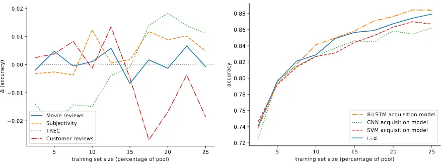
Figure 1: We highlight practical issues in the use of AL. (a) AL yields inconsistent gains, relative to a baseline of i.i.d. sampling, across corpora. (b) Training a BiLSTM with training sets actively acquired based on the uncertainty of other models tends to result in worse performance than training on i.i.d. samples.

In contrast to experimental (retrospective) stud-ies, in a real-world setting, an AL practitioner is not afforded the opportunity to retrospectively an-alyze or alter their scoring function. One would instead need to expend significant resources to val-idate that a given scoring function performs as in-tended for a particular model and task. This would require i.i.d. sampled data to evaluate the com-parative effectiveness of different AL strategies. However, collection of such additional data would defeat the purpose of AL, i.e., obviating the need for a large amount of supervision. To confidently use AL in practice, one must have a reasonable be-lief that a given AL scoring (oracquisition) func-tion will produce the desired resultsbefore they de-ploy it(Attenberg and Provost,2011).

Most AL research does not explicitly character-ize the circumstances under which AL may be ex-pected to perform well. Practitioners must there-fore make the implicit assumption that a given ac-tive acquisition strategy is likely to perform well under anycircumstances. Our empirical findings suggest that this assumption is not well founded and, in fact, common AL algorithms behave in-consistently across model types and datasets, of-ten performing no better than random (i.i.d.) sam-pling (1a). Further, while there is typicallysome

AL strategy which outperforms i.i.d. random sam-ples for a given dataset,whichheuristic varies.

Contributions. We highlight important but of-ten overlooked issues in the use of AL in practice. We report an extensive set of experimental results on classification and sequence tagging tasks that

suggest AL typically affords only marginal per-formance gains at the somewhat high cost of non-i.i.d. training samples, which do not consistently transfer well to subsequent models.

2 The (Potential) Trouble with AL

We illustrate inconsistent comparative perfor-mance using AL. Consider Figure 1a, in which we plot the relative gains (∆) achieved by a BiLSTM model using a maximum-entropy active sampling strategy, as compared to the same model trained with randomly sampled data. Positive val-ues on the y-axis correspond to cases in which AL achieves better performance than random sam-pling, 0 (dotted line) indicates no difference be-tween the two, and negative values correspond to cases in which random sampling performs better than AL. Across the four datasets shown, results are decidedly mixed.

ques-tions arise: How does a successormodel S fare, when trained on data collected via an acquisition modelA? How does this compare to trainingSon natively acquired data? How does it compare to trainingSon i.i.d. data?

For example, if we use uncertainty sampling un-der a support vector machine (SVM) to acquire a training setD, and subsequently train a Convolu-tional Neural Network (CNN) using D, will the CNN perform better than it would have if trained on a dataset acquired via i.i.d. random sampling? And how does it perform compared to using a training corpus actively acquired using the CNN?

Figure 1b shows results for a text classifica-tion example using the Subjectivity corpus (Pang and Lee, 2004). We consider three models: a Bidirectional Long Short-Term Memory Network (BiLSTM) (Hochreiter and Schmidhuber, 1997), a Convolutional Neural Network (CNN) (Kim,

2014;Zhang and Wallace, 2015), and a Support Vector Machine (SVM) (Joachims,1998). Train-ing the LSTM with a dataset actively acquired us-ing either of the other models yields predictive performance that isworsethan that achieved under i.i.d. sampling. Given that datasets tend to outlast models, these results raise questions regarding the benefits of using AL in practice.

We note that in prior work,Tomanek and Morik

(2011) also explored the transferability of actively acquired datasets, although their work did not con-sider modern deep learning models or share our broader focus on practical issues in AL.

3 Experimental Questions and Setup

We seek to answer two questions empirically: (1) How reliably does AL yield gains over sampling i.i.d.? And, (2) What happens when we use a dataset actively acquired using one model to train a different (successor) model? To answer these questions, we consider two tasks for which AL has previously been shown to confer considerable benefits: text classification and sequence tagging (specifically NER).2

To build intuition, our experiments address both linear models and deep networks more representa-tive of the current state-of-the-art for these tasks. We investigate the standard strategy of acquiring data and training using a single model, and also

2_{Recent works have shown that AL is effective for these} tasks even when using modern, neural architectures (Zhang et al.,2017;Shen et al.,2018), but do not address our primary concerns regarding replicability and transferability.

the case of acquiring data using one model and subsequently using it to train a second model. Our experiments consider all possible (acquisi-tion, successor) pairs among the considered mod-els, such that the standard AL scheme corresponds to the setting in which the acquisition and succes-sor models are same. For each pair (A, S), we first simulate iterative active data acquisition with modelAto label a training datasetDA. We then train the successor modelSusingD_A.

In our evaluation, we compare the relative per-formance (accuracy or F1, as appropriate for the task) of the successor model trained with corpus

DAto the scores achieved by training on compara-ble amounts of native and i.i.d. sampled data. We simulate pool-based AL using labeled benchmark datasets by withholding document labels from the models. This induces a pool of unlabeled data

U. In AL, it is common to warm-start the ac-quisition model, training on some modest amount of i.i.d. labeled data D_w before using the model to score candidates inU (Settles,2009) and com-mencing the AL process. We follow this conven-tion throughout.

Once we have trained the acquisition model on the warm-start data, we begin the simulated AL loop, iteratively selecting instances for labeling and adding them to the dataset. We denote the dataset acquired by modelAat iterationtbyDt

A;

D0

Ais initialized toDwfor all models (i.e., all val-ues ofA). At each iteration, the acquisition model is trained withDt

A. It then scores the remaining unlabeled documents in U \ Dt

A according to a standard uncertainty AL heuristic. The topn can-didatesCt

Aare selected for (simulated) annotation. Their labels are revealed and they are added to the training set: Dt_A+1 ← Dt

A∪ CAt. At the experi-ment’s conclusion (time stepT), each acquisition model A will have selected a (typically distinct) subset ofU for training.

Once we have acquired datasets from each ac-quisition modelDA, we evaluate the performance of each possible successor model when trained on

DA. Specifically, we train each successor model

S on the acquired data Dt

A for all t in the range

[0, T], evaluating its performance on a held-out test set (distinct fromU). We compare the perfor-mance achieved in this case to that obtained using an i.i.d. training set of the same size.

in Figure 1. All reported results, including i.i.d. baselines, are averages of ten experiments, each conducted with a distinct Dw. These learning curves quantify the comparative performance of a particular model achieved using the same amount of supervision, but elicited under different acqui-sition models. For each model, we compare the learning curves of each acquisition strategy, in-cluding active acquisition using a foreignmodel and subsequent transfer, active acquisition without changing models (i.e., typical AL), and the base-line strategy of i.i.d. sampling.

4 Tasks

We now briefly describe the models, datasets, ac-quisition functions, and implementation details for the experiments we conduct with active learners for text classification (4.1) and NER (4.2).

4.1 Text Classification

Models We consider three standard models for text classification: Support Vector Machines (SVMs), Convolutional Neural Networks (CNNs) (Kim,2014;Zhang and Wallace,2015), and Bidi-rectional Long Short-Term Memory (BiLSTM) networks (Hochreiter and Schmidhuber, 1997). For SVM, we represent texts via sparse, TF-IDF bag-of-words (BoW) vectors. For neural models (CNN and BiLSTM), we represent each document as a sequence of word embeddings, stacked into an

l×dmatrix wherelis the length of the sentence and d is the dimensionality of the word embed-dings. We initialize all word embeddings with pre-trained GloVe vectors (Pennington et al.,2014).

We initialize vector representations for all words for which we do not have pre-trained em-beddings uniformly at random. For the CNN, we impose a maximum sentence length of 120

words, truncating sentences exceeding this length and padding shorter sentences. We used filter sizes of3,4, and5, with 128filters per size. For BiL-STMs, we selected the maximum sentence length such that 90% of sentences in Dt _{would be of} equal or lesser length.3 We trained all neural mod-els using the Adam optimizer (Kingma and Ba,

2014), with a learning rate of 0.001, β1 = 0.9,

β1 = 0.999, and= 10−8.

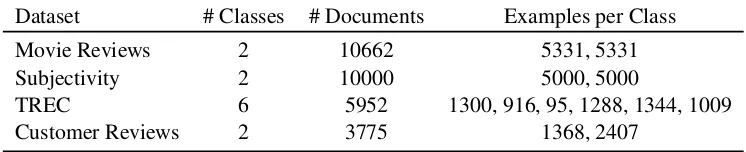
Datasets We perform text classification experi-ments using four benchmark datasets. We reserve

3_{Passing longer sentences to the BiLSTM degraded} per-formance in preliminary experiments.

20%of each dataset (sampled at i.i.d. random) as test data, and use the remaining80%as the pool of unlabeled dataU. We sample2.5%of the remain-ing documents randomly fromU for eachDw. All models receive the sameDw for any given experi-ment.

• Movie Reviews: This corpus consists of sen-tences drawn from movie reviews. The task is to classify sentences as expressing positive or negative sentiment (Pang and Lee,2005).

• Subjectivity: This dataset consists of state-ments labeled as either objective or subjective (Pang and Lee,2004).

• TREC: This task entails categorizing questions into 1 of 6 categories based on the subject of the question (e.g., questions about people, lo-cations, and so on) (Li and Roth, 2002). The TREC dataset defines standard train/test splits, but we generate our own for consistency in train/validation/test proportions across corpora.

• Customer Reviews: This dataset is composed of product reviews. The task is to categorize them as positive or negative (Hu and Liu,2004).

4.2 Named Entity Recognition

Models We consider transfer between two NER models: Conditional Random Fields (CRF) ( Laf-ferty et al.,2001) and Bidirectional LSTM-CNNs (BiLSTM-CNNs) (Chiu and Nichols,2015).

For the CRF model we use a set of fea-tures including word-level and character-based embeddings, word suffix, capitalization, digit con-tents, and part-of-speech tags. The BiLSTM-CNN model4 initializes word vectors to pre-trained GloVe vector embeddings (Pennington et al., 2014). We learn all word and character level features from scratch, initializing with ran-dom embeddings.

Datasets We perform NER experiments on the CoNLL-2003 and OntoNotes-5.0 English datasets. We used the standard test sets for both corpora, but merged training and validation sets to formU. We initialize eachD_w to2.5%ofU.

• CoNLL-2003: Sentences from Reuters news with words tagged as person, location, organi-zation, or miscellaneous entities using an IOB

5 10 15 20 25 training set size (percentage of pool) 0.60

0.62 0.64 0.66 0.68 0.70

accuracy

BiLSTM acquisition model CNN acquisition model SVM acquisition model i.i.d.

(a) SVM on Movies dataset

5 10 15 20 25

training set size (percentage of pool) 0.58

0.60 0.62 0.64 0.66 0.68 0.70

accuracy

(b) CNN on Movies dataset

5 10 15 20 25

training set size (percentage of pool) 0.56

0.58 0.60 0.62 0.64 0.66 0.68

accuracy

(c) LSTM on Movies dataset

5 10 15 20 25

training set size (percentage of pool) 62.5

65.0 67.5 70.0 72.5 75.0 77.5 80.0

F1

BiLSTM-CNN acquisition model CRF acquisition model i.i.d.

(d) CRF on OntoNotes dataset

5 10 15 20 25

training set size (percentage of pool) 76

78 80 82 84 86

F1

(e) BiLSTM-CNN on OntoNotes dataset

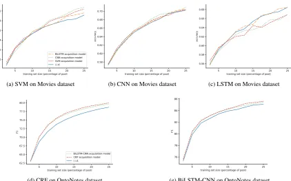
Figure 2: Sample learning curves for the text classification task on the Movie Reviews dataset and the NER task on the OntoNotes dataset using the maximum entropy acquisition function (we report learning curves for all models and datasets in the Appendix). Individual plots correspond to successor models. Each line corresponds to an acquisition model, with the blue line representing an i.i.d. baseline.

scheme (Tjong Kim Sang and De Meulder,

2003). The corpus contains 301,418 words.

• OntoNotes-5.0: A corpus of sentences drawn from a variety of sources including newswire, broadcast news, broadcast conversation, and web data. Words are categorized using eigh-teen entity categories annotated using the IOB scheme (Weischedel et al., 2013). The corpus contains 2,053,446 words.

4.3 Acquisition Functions

We evaluate these models using three common ac-tive learning acquisition functions: classical un-certainty sampling, query by committee (QBC), and Bayesian active learning by disagreement (BALD).

Uncertainty Sampling For text classification we use the entropy variant of uncertainty sam-pling, which is perhaps the most widely used AL heuristic (Settles,2009). Documents are selected for annotation according to the function

argmax

x∈U

−X

j

P(yj|x) logP(yj|x),

wherexare instances in the pool U,j indexes potential labels of these (we have elided the

in-stance index here) and P(yj|x) is the predicted probability that x belongs to class yj (this esti-mate is implicitly conditioned on a model that can provide such estimates). For SVM, the equivalent form of this is to choose documents closest to the decision boundary.

For the NER task we use maximized normal-ized log-probability (MNLP) (Shen et al., 2018) as our AL heuristic, which adapts the least confi-dence heuristics to sequences by normalizing the log probabilities of predicted tag sequence by the sequence length. This avoids favoring selecting longer sentences (owing to the lower probability of getting the entire tag sequence right).

Documents are sorted in ascending order ac-cording to the function

max

y1,...,yn

1 n

n X

i=1

logP(yi|y1, ..., yn−1,x)

Text classification

Acquisition model

10% of pool 20% of pool

Successor i.i.d. SVM CNN LSTM i.i.d. SVM CNN LSTM

Movie reviews

SVM 65.3 65.3 65.8 65.7 68.2 69.0 69.4 68.9

CNN 65.0 65.3 65.5 65.4 69.4 69.1 69.5 69.5

LSTM 63.0 62.0 62.5 63.1 67.2 65.1 65.8 67.0

Subjectivity

SVM 85.2 85.6 85.3 85.5 87.5 87.6 87.4 87.6

CNN 85.3 85.2 86.3 86.0 87.9 87.6 88.4 88.6

LSTM 82.9 82.7 82.7 84.1 86.7 86.3 85.8 87.6

TREC

SVM 68.5 68.3 66.8 68.5 74.1 74.7 73.2 74.3

CNN 70.9 70.5 69.0 70.0 76.1 77.7 77.3 78.0

LSTM 65.2 64.5 63.6 63.8 71.5 72.7 71.0 73.3

Customer reviews

SVM 68.8 70.5 70.3 68.5 73.6 74.2 72.9 71.1

CNN 70.6 70.9 71.7 68.2 74.1 74.5 74.8 71.5

LSTM 66.1 67.2 65.1 65.9 68.0 66.6 66.5 66.3

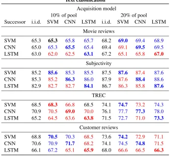
Table 1: Text classification accuracy, evaluated for each combination of acquisition and successor models using uncertainty sampling. Accuracies are reported for training sets composed of 10% and 20% of the document pool. Colors indicate performance relative to i.i.d. baselines: Blue indicates that a model fared better, red that it performed worse, and black that it performed the same.

Named Entity Recognition

Acquisition Model

10% of pool 20% of pool

Successor i.i.d. CRF BiLSTM-CNN i.i.d. CRF BiLSTM-CNN

CoNLL

CRF 69.2 70.5 70.2 73.6 74.4 74.0

BiLSTM-CNN 87.4 87.4 87.8 89.1 89.6 89.6

OntoNotes

CRF 73.8 75.5 75.4 77.6 79.1 78.7

BiLSTM-CNN 82.6 83.1 83.1 84.6 85.2 84.9

Table 2: F1 measurements for the NER task, with training sets comprising 10% and 20% of the training pool.

Query by Committee For our QBC experi-ments, we use the bagging variant of QBC (Mamitsuka et al.,1998), in which a committee of

nmodels is assembled by sampling with replace-mentnsets ofmdocuments from the training data (Dt_{at eacht). Each model is then trained using a} distinct resulting set, and the pool documents that

maximize their disagreement are selected. We use

10as our committee size, and setmas equal to the number of documents inDt_.

docu-Dataset # Classes # Documents Examples per Class

Movie Reviews 2 10662 5331, 5331

Subjectivity 2 10000 5000, 5000

TREC 6 5952 1300, 916, 95, 1288, 1344, 1009

Customer Reviews 2 3775 1368, 2407

Table 3: Text classification dataset statistics.

ments for annotation according to the function

argmax

x∈U 1 C

C X

c=1

X

j

Pc(yj|x) log

Pc(yj|x)

PC(yj|x)

where x are instances in the pool U, j in-dexes potential labels of these instances, and C

is the committee size. Pc(yj|x) is the proba-bility that x belongs to class yj as predicted by committee member c. PC(yj|x) represents the consensus probability that x belongs to class yj,

1

C

PC

c=1Pc(yj|x).

For NER, we compute disagreement using the average per word vote-entropy (Dagan and En-gelson,1995), selecting sequences for annotation which maximize the function

−1

n

n X

i=1

X

m

V(yi, m)

C log

V(yi, m)

C

where nis the sequence length,C is the com-mittee size, and V(yi, m) is the number of com-mittee members who assign tag m to word i in their most likely tag sequence. We do not apply the QBC acquisition function to the OntoNotes dataset, as training the committee for this larger dataset becomes impractical.

Bayesian AL by Disagreement We use the Monte Carlo variant of BALD, which exploits an interpretation of dropout regularization as a Bayesian approximation to a Gaussian process (Gal et al., 2017b; Siddhant and Lipton, 2018). This technique entails applying dropout at test time, and then estimating uncertainty as the dis-agreement between outputs realized via multiple passes through the model. We use the acquisition function proposed in (Siddhant and Lipton,2018), which selects for annotation those instances that maximize the number of passes through the model that disagree with the most popular choice:

argmax

x∈U

(1−count(mode(y

1

x, ..., yTx))

T )

where xare instances in the pool U, yi_x is the class prediction of theith model pass on instance

x, and T is the number of passes taken through the model. Any ties are resolved using uncertainty sampling over the mean predicted probabilities of allT passes.

In the NER task, agreement is measured across the entire sequence. Because this acquisition func-tion relies on dropout, we do not consider it for non-neural models (SVM and CRF).

5 Results

We compare transfer between all possible (acqui-sition, successor) model pairs for each task. We report the performance of each model under all ac-quisition functions both in tables compiling results (Table 1 and Table 2for classification and NER, respectively) and graphically via learning curves that plot predictive performance as a function of train set size (Figure2).

We report additional results, including all learn-ing curves (for all model pairs and for all tasks), and tabular results (for all acquisition functions) in the Appendix. We also provide in the Ap-pendix plots resembling1a for all (model, acqui-sition function) pairs that report the difference be-tween performance under standard AL (in which acquisition and successor model are the same) and that under commensurate i.i.d. data, which affords further analysis of the gains offered by standard AL. For text classification tasks, we report accura-cies; for NER tasks, we report F1.

To compare the learning curves, we select in-cremental points along the x-axis and report the performance at these points. Specifically, we re-port results with training sets containing 10% and 20% of the training pool.

6 Discussion

incon-Successor

Movie Reiews Subjectivity TREC Customer Reviews

Acquisition Model CNN LSTM CNN LSTM CNN LSTM CNN LSTM

CNN – 0.961 – 0.968 – 0.988 – 0.973

LSTM 0.989 – 0.996 – 0.992 – 0.980 –

SVM 0.991 0.961 0.997 0.970 0.990 0.987 0.991 0.974

Table 4: Average Spearman’s rank correlation coefficients (over five runs) of cosine distances between test set representations learned with native active learning and distances between those learned with transferred actively acquired datasets, at the end of the AL process. Uncertainty is used as the acquisition function in all cases.

sistently across text classification datasets. In75%

of all combinations of model, dataset, and training set size, there exists some acquisition function that outperforms i.i.d. data. This is consistent with the prior literature indicating the effectiveness of AL. However, when implementing AL in a real, live setting, a practitioner would choose asingle acqui-sition function ahead of time. To accurately reflect this scenario, we must consider the performance of individual acquisition functions across multiple datasets. Results for individual AL strategies are more equivocal. In our reported classification dat-apoints, standard AL outperforms i.i.d. sampling in only a slight majority (60.9%) of cases.

AL thus seems to yield modest (though incon-sistent) improvements over i.i.d. random sam-pling, but our results further suggest that this comes at an additional cost: the acquired dataset may not generalize well to new learners. Specifi-cally, models trained onforeignactively acquired datasets tend to underperform those trained on i.i.d. datasets. We observe this most clearly in the classification task, where only a handful of (acquisition, successor, acquisition function) com-binations lead to performance greater than that achieved using i.i.d. data. Specifically, only 37.5% of the tabulated data points representing dataset transfer (in which acquisition and succes-sor models differ) outperform the i.i.d. baseline.

Results for NER are more favorable for AL. For this task we observe consistent improved perfor-mance versus the i.i.d. baseline in both standard AL data points and transfer data points. These results are consistent with previous findings on transferring actively acquired datasets for NER (Tomanek and Morik,2011).

In standard AL for text classification, the only (model, acquisition function) pairs that we observe to produce better than i.i.d. results with any reg-ularity are uncertainty with SVM or CNN, and

BALD with CNN. When transferring actively ac-quired datasets, we do not observe consistently better than i.i.d. results withanycombination of acquisition model, successor model, and acqui-sition function. The success of AL appears to depend very much on the dataset. For example, AL methods – both in the standard and acquisi-tion/successor settings – perform much more reli-ably on the Subjectivity dataset than any other. In contrast, AL performs consistently poorly on the TREC dataset.

Our findings suggest that AL is brittle. Dur-ing experimentation, we also found that perfor-mance often depends on factors that one may think are minor design decisions. For example, our setup largely resembles that ofSiddhant and Lip-ton (2018), yet initially we observed large dis-crepancies in results. Digging into this revealed that much of the difference was due to our use of word2vec (Mikolov et al.,2013) rather than GloVe (Pennington et al.,2014) for word embedding ini-tializations. That small decisions like this can re-sult in relatively pronounced performance differ-ences for AL strategies is disconcerting.

A key advantage afforded by neural models is representation learning. A natural question here is therefore whether the representations induced by the neural models differs as a function of the acquisition strategy. To investigate this, we mea-sure pairwise distances between instances in the learned feature space after training. Specifically, for each test instance we calculate its cosine sim-ilarity to all other test instances, inducing a rank-ing. We do this in the three different feature spaces learned by the CNN and LSTM models, respec-tively, after sampling under the three acquisition models.

re-peat this for all instances in the test set, and aver-age over these coefficients to derive an overall sim-ilarity measure, which may be viewed as quantify-ing the similarity between learned feature spaces via average pairwise similarities within them. As reported in Table 4, despite the aforementioned differences in predictive performance, the learned representations seem to be similar. In other words, sampling under foreign acquisition models does not lead to notably different representations.

7 Conclusions

We extensively evaluated standard AL methods under varying model, domain, and acquisition function combinations for two standard NLP tasks (text classification and sequence tagging). We also assessed performance achieved when transferring an actively sampled training dataset from an acqui-sition model to a distinct successor model. Given the longevity and value of training sets and the frequency at which new ML models advance the state-of-the-art, this should be an anticipated sce-nario: Annotated data often outlives models.

Our findings indicate that AL performs unreli-ably. While a specific acquisition function and model applied to a particular task and domain may be quite effective, it is not clear that this can be predicted ahead of time. Indeed, there is no way to retrospectively determine the relative success of AL without collecting a relatively large quantity of i.i.d. sampled data, and this would undermine the purpose of AL in the first place. Further, even if such an i.i.d. sample were taken as a diagnos-tic tool early in the active learning cycle, relative success early in the AL cycle is not necessarily in-dicative of relative success later in the cycle, as illustrated by Figure1a.

Problematically, even in successful cases, an ac-tively sampled training set is linked to the model used to acquire it. We have found that training successor models with this set will often result in performance worse than that attained using an equivalently sized i.i.d. sample. Results are more favorable to AL for NER, as compared to text classification, which is consistent with prior work (Tomanek and Morik,2011).

In short, the relative performance of individ-ual active acquisition functions varies consider-ably over datasets and domains. While AL of-ten does yield gains over i.i.d. sampling, these tend to be marginal and inconsistent. Moreover,

this comes at a relatively steep cost: The acquired dataset may be disadvantageous for training sub-sequent models. Together these findings raise seri-ous concerns regarding the efficacy of active learn-ing in practice.

8 Acknowledgements

This work was supported in part by the Army Re-search Office (ARO), award W911NF1810328.

References

Josh Attenberg and Foster Provost. 2011. Inactive

learning?: difficulties employing active learning in

practice. ACM SIGKDD Explorations Newsletter,

12(2):36–41.

Olivier Chapelle, Bernhard Scholkopf, and Alexander Zien. 2009. Semi-supervised learning (chapelle, o. et al., eds.; 2006)[book reviews]. IEEE Transactions on Neural Networks, 20(3):542–542.

Jason PC Chiu and Eric Nichols. 2015. Named en-tity recognition with bidirectional lstm-cnns. arXiv preprint arXiv:1511.08308.

David A Cohn, Zoubin Ghahramani, and Michael I Jor-dan. 1996. Active learning with statistical models.

Journal of artificial intelligence research, 4:129– 145.

Ido Dagan and Sean P Engelson. 1995. Committee-based sampling for training probabilistic classifiers. InMachine Learning Proceedings 1995, pages 150– 157. Elsevier.

Yarin Gal, Riashat Islam, and Zoubin Ghahramani.

2017a. Deep bayesian active learning with

im-age data. InInternational Conference on Machine

Learning, pages 1183–1192.

Yarin Gal, Riashat Islam, and Zoubin Ghahramani.

2017b. Deep bayesian active learning with image

data.CoRR, abs/1703.02910.

Abbas Ghaddar and Phillippe Langlais. 2018. Robust

lexical features for improved neural network named-entity recognition. In Proceedings of the 27th In-ternational Conference on Computational

Linguis-tics, pages 1896–1907. Association for

Computa-tional Linguistics.

Sepp Hochreiter and J¨urgen Schmidhuber. 1997.

Long short-term memory. Neural computation,

9(8):1735–1780.

Thorsten Joachims. 1998. Text categorization with support vector machines: Learning with many

rel-evant features. InEuropean conference on machine

learning, pages 137–142. Springer.

Rie Johnson and Tong Zhang. 2016. Supervised and

semi-supervised text categorization using lstm for region embeddings. InProceedings of the 33rd In-ternational Conference on InIn-ternational Conference on Machine Learning - Volume 48, ICML’16, pages 526–534. JMLR.org.

Yoon Kim. 2014. Convolutional neural

net-works for sentence classification. arXiv preprint

arXiv:1408.5882.

Diederik P Kingma and Jimmy Ba. 2014. Adam: A

method for stochastic optimization. arXiv preprint

arXiv:1412.6980.

John D. Lafferty, Andrew McCallum, and Fernando

C. N. Pereira. 2001. Conditional random fields:

Probabilistic models for segmenting and labeling se-quence data. InProceedings of the Eighteenth Inter-national Conference on Machine Learning, ICML ’01, pages 282–289, San Francisco, CA, USA. Mor-gan Kaufmann Publishers Inc.

Xin Li and Dan Roth. 2002. Learning question

clas-sifiers. In Proceedings of the 19th international

conference on Computational linguistics-Volume 1, pages 1–7. Association for Computational Linguis-tics.

Naoki Abe Hiroshi Mamitsuka et al. 1998. Query

learning strategies using boosting and bagging. In

Machine learning: proceedings of the fifteenth inter-national conference (ICML98), volume 1. Morgan Kaufmann Pub.

Andrew Kachites McCallum and Kamal Nigamy. 1998. Employing em and pool-based active learning for text classification. In Proc. International Confer-ence on Machine Learning (ICML), pages 359–367. Citeseer.

Tomas Mikolov, Kai Chen, Greg Corrado, and Jeffrey

Dean. 2013. Efficient estimation of word

represen-tations in vector space.

Sinno Jialin Pan and Qiang Yang. 2010. A survey on

transfer learning. IEEE Transactions on knowledge

and data engineering, 22(10):1345–1359.

Bo Pang and Lillian Lee. 2004. A sentimental educa-tion: Sentiment analysis using subjectivity

summa-rization based on minimum cuts. InProceedings of

the ACL.

Bo Pang and Lillian Lee. 2005. Seeing stars: Exploit-ing class relationships for sentiment categorization with respect to rating scales. InProceedings of the ACL.

Jeffrey Pennington, Richard Socher, and

Christo-pher D. Manning. 2014. Glove: Global vectors for

word representation. InEmpirical Methods in Nat-ural Language Processing (EMNLP), pages 1532– 1543.

Maria E. Ramirez-Loaiza, Manali Sharma, Geet Ku-mar, and Mustafa Bilgic. 2017. Active learning: an empirical study of common baselines. Data Mining and Knowledge Discovery, 31(2):287–313.

B. Settles. 2009. Active learning literature survey. Computer Sciences Technical Report 1648, Univer-sity of Wisconsin–Madison.

Burr Settles. 2012. Active learning. Synthesis

Lec-tures on Artificial Intelligence and Machine Learn-ing, 6(1):1–114.

Yanyao Shen, Hyokun Yun, Zachary C. Lipton, Yakov Kronrod, and Animashree Anandkumar. 2018. Deep active learning for named entity recog-nition. In International Conference on Learning Representations.

Aditya Siddhant and Zachary C Lipton. 2018. Deep bayesian active learning for natural language pro-cessing: Results of a large-scale empirical study.

arXiv preprint arXiv:1808.05697.

Erik F. Tjong Kim Sang and Fien De Meulder. 2003. Introduction to the conll-2003 shared task: Language-independent named entity recognition. In

Proceedings of CoNLL-2003, pages 142–147. Ed-monton, Canada.

Katrin Tomanek and Katharina Morik. 2011.

Inspect-ing sample reusability for active learnInspect-ing. In

Ac-tive Learning and Experimental Design workshop In conjunction with AISTATS 2010, pages 169–181.

Ralph Weischedel, Martha Palmer, Mitchell Marcus, Eduard Hovy, Sameer Pradhan, Lance Ramshaw, Nianwen Xue, Ann Taylor, Jeff Kaufman, Michelle

Franchini, et al. 2013. Ontonotes release 5.0

ldc2013t19. Linguistic Data Consortium,

Philadel-phia, PA.

Ye Zhang, Matthew Lease, and Byron C Wallace. 2017. Active discriminative text representation learning. InAAAI.