Transformation Using Neural-Based Identification for Controlling
Singularly-Perturbed Eigenvalue-Preserved Reduced Order Systems
Anas N. Al-Rabadi and Othman M.K. Alsmadi
Abstract - This paper introduces a new hierarchy for controlling dynamical systems. The new control hierarchy uses supervised neural network to identify certain parameters of the transformed system matrix [A~]. Then, Linear Matrix Inequality (LMI) is used to determine the permutation matrix [P] so that a complete system transformation {[B~], [C~], [D~]} is performed. The transformed model is then reduced using singular perturbation method, and various feedback control schemes are applied to enhance system performance, including PID control, state feedback control using pole assignment, state feedback control using LQR optimal control, and output feedback control. The comparative experimental results between system transformation without using LMI and state transformation via using LMI shows clearly the superiority in system modeling and control using the proposed LMI-based control method. The new control methodology simplifies the system model and thus uses simpler controllers to produce the desired response.
Index Terms - Linear Matrix Inequality (LMI), LQR Optimal Control, Neural Networks, Order Model Reduction, Output Feedback Control, PID Control, Parameter Estimation, Pole Placement, Singular Perturbation Methods, State Feedback Control, System Identification.
1. INTRODUCTION
The general objective of control systems is to cause the output variable of a dynamic process to follow the desired reference variable accurately. This goal can be achieved based on a number of steps. An important one is to develop a mathematical model to be controlled [4,6]. This model is usually done using a set of differential equations that describe the system dynamic behavior.
In system modeling, sometimes it is required to identify certain parameters. This objective maybe achieved by the use of artificial neural networks (ANN) [8,9,15,16]. Artificial neural systems maybe defined as physical cellular systems which have the capability of acquiring, storing and utilizing experiential knowledge [8,16]. It consists of an interconnected group of artificial neurons and processes information using a computational connectionist approach. The basic processing elements of neural networks are called neurons. They perform summing operations and nonlinear functions. Neurons are usually organized in layers and forward connections and computations are performed in a parallel fashion at all nodes and connections.
A. N. Al-Rabadi is with the Computer Engineering Department, The University of Jordan, Amman, Jordan (Phone: + 962-79-644-5364; E-mail: [email protected]; URL: http://web.pdx.edu/~psu21829/) O. M.K. Alsmadi is with the Electrical Engineering Department, The University of Jordan, Amman, Jordan (E-mail: [email protected])
Each ANN connection is expressed by a numerical value called a weight. The learning process of a neuron corresponds to a way of changing its weights. In fact, they can be used to model complex relationships between inputs and outputs or to find patterns in data [2,8,9,15,16].
When dealing with system modeling and control analysis, some equations and inequalities require optimized solutions. A numerical algorithm called Linear Matrix Inequality (LMI) serves as an optimization technique [1,3]. The LMI started by the Lyapunov theory showing that the differential equation x&(t)=Ax(t) is stable if and only if there exists a positive definite matrix [P] such that ATP+PA<0
[3]. The requirement P>0, ATP+PA<0 is what is known as Lyapunov inequality on [P] which is a special case of an
LMI. By picking any Q=QT >0 and then solving the linear equation ATP+PA=−Qfor the matrix [P], it is guaranteed
to be positive-definite if the given system is stable [3]. In practical control design problems, the first step is to obtain a mathematical model in order to examine the system behavior for the purpose of designing a proper controller [1,2,3,4,5,7,9,11,12,13,14]. Sometimes, this mathematical description involves a certain small parameter (perturbation). Neglecting this small parameter results in reducing the order model of the system and thus simplifying the controller design [1,2,5,7,9,11,12,13,14]. A reduced order model can be obtained by neglecting the fast dynamics (i.e., non-dominant eigenvalues) of the system and focusing on the slow dynamics (i.e., dominant eigenvalues). This model reduction leads to controller cost minimization [4,6,7]. In control system, due to the fact that feedback controllers do not usually consider all the dynamics of the system, model reduction is a very important issue [2,9]. One of the model reduction methods is the singular perturbation [5,7,11,14].
0
k
w
1
k
w
2
k
w
∑
ϕ
(
•)
ky
1
x
2
x
p
x
Output Activation Function
Summing Junction
Synaptic Weights Input
Signals
k
v
Threshold
k
θ
kp
w
0
x
Continuous Dynamic System: {[A], [B], [C], [D]}
System Discretization
System Undiscretization (Continuous)
LMI-Based Permutation matrix [P]
Order Model Reduction
Output Feedback Control
(LQR-Based Control)
PID Control
LQR Optimal Control
Pole Placement
Closed-Loop Feedback Control
Complete System
Transformation: {[B~],[C~],[D~]}
State Feedback Control
Neural-Based System
Transformation:{[Aˆ ],[ Bˆ ]}
Neural-Based State
Transformation:[A~]
[image:2.612.131.462.51.312.2]
Figure 1. The new hierarchical control methodology used in this paper.
2. FUNDAMENTALS
The following sections provide an important background which will be used Sections 3-5.
2.1 Recurrent Supervised Neural Network
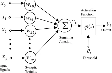
An artificial NN is an emulation of a biological neural system. The process of a neuron may be mathematically modeled as shown in Figure 2 [8,16].
Figure 2. Mathematical model of an artificial neuron.
As seen in Figure 2, the internal activity of the neuron is:
∑
= =
p
j
j kj
k w x
v 1
(1) In supervised learning, it is assumed that at each instant of time when the input is applied, the desired response of the
system is available [8,16]. The difference between the actual and the desired response represents an error measure and is used to correct the network parameters externally. Since the adjustable weights are initially assumed, the error measure may be used to adapt the network's weight matrix [W]. A
set of input and output patterns is required for this learning mode. The training algorithm estimates the negative error gradient directions and reduces the resulting error [8,16].
The supervised NN used for identification in this paper is based on an approximation of the method of steepest descent [8,15,16]. The network tries to match the output of certain neurons to the desired values of the system output at specific instant of time.
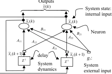
Consider a network consisting of a total of N
neurons with M external input connections, as shown in Figure 3 for a 2nd order system with two neurons and one external input. The variable g(k) denotes the (M x 1) external
input vector applied to the network at discrete time k. The variable y(k + 1) denotes the corresponding (N x 1) vector of
individual neuron outputs produced one step later at time (k + 1). The input vector g(k) and one-step delayed output
vector y(k) are concatenated to form the ((M + N) x 1) vector u(k), whose ith element is denoted by ui(k). IfΛ denotes the
set of indices i for which gi(k) is an external input, and β
denotes the set of indices i for which ui(k) is the output of a
neuron (which is yi(k)), the following is true:
⎪⎩ ⎪ ⎨ ⎧
∈ ∈
β
i , k y
Λ
i , k g = k u
i i i
if ) (
if ) ( )
(
[image:2.612.71.293.464.608.2]Z-1 g1:
A11 A12
A21 A22 B11 B21 ) 1 ( ~
1 k+
x System external input System dynamics System state: internalinput Neuron delay Z-1 Outputs ~y(k)
) 1 ( ~
2 k+
x )
( ~
1k
x ~x2(k)
[image:3.612.53.281.57.209.2]4
4 8
4
4 7
6
Figure 3. A second order recurrent neural network architecture,
where the estimated matrices are given by: ⎥
⎦ ⎤ ⎢ ⎣ ⎡ = 22 21 12 11 ~ A A A A
Ad ,
⎥ ⎦ ⎤ ⎢ ⎣ ⎡ = 21 11 ~ B B
Bd and that W=
[
[A~d] [B~d]]
.neuron j at time k is given by: ) ( ) ( = )
(k w k u k
v ji i
Λ i
j
∑
∪
∈ β
where Λ ∪ ßis the union of sets Λand ß. At the next time step (k + 1), the output of the neuron j is computed by passing vj(k) through the nonlinearity ϕ(.) obtaining:
)) ( ( = ) 1
(k v k
yj + ϕ j
The derivation of the recurrent algorithm can be started by using dj(k) to denote the desired (target) response
of neuron j at time k, and ς(k) to denote the set of neurons that are chosen to provide externally reachable outputs. A time-varying (N x 1) error vector e(k) is defined whose jth
element is given by the following relationship:
⎪⎩ ⎪ ⎨ ⎧ ∈ otherwise 0, ) ( if ), ( ) ( = )
(k d k y k j k
ej j j ς
The objective is to minimize the cost function Etotal which is: )
( =
total E k
E
k
∑
, where ( )2 1 = )
(k e2 k
E j
j
∑
∈ς
To accomplish this objective, the steepest descent is used:
= total = ( )= ( )
total E k E k
E E k k W W W
W ∂ ∇
∂ ∂
∂
∇
∑
∑
where∇WE(k) is the gradient of E(k) with respect to the weight matrix [W]. In order to train the recurrent network in
real time, the instantaneous estimate of the gradient is used
(
∇WE(k))
. For the case of a particular weight wml(k), theincremental change Δwml(k) made at time k is defined as: ) ( ) ( -= ) ( k w k E k w m m l l ∂ ∂ Δ η
where η is the learning-rate parameter. Hence:
) ( ) ( ) ( -= ) ( ) ( ) ( = ) ( ) ( k w k y k e k w k e k e k w k E m i j j m j j j
ml l ∂ l
∂ ∂ ∂ ∂ ∂
∑
∑
∈∈ς ς
To determine the partial derivative ∂yj(k)/∂wml(k), the network dynamics are derived. The derivation is obtained by using the chain rule which provides the following equation: ) ( ) ( )) ( ( ) ( ) ( ) ( 1) + ( = ) ( 1) + ( k w k v k v k w k v k v k y k w k y m j j m j j j m j l l l & ∂ ∂ = ∂ ∂ ∂ ∂ ∂ ∂ ϕ where ) ( )) ( ( = )) ( ( k v k v k v j j j ∂ ∂ϕ
ϕ& .
Differentiating the net internal activity of neuron j with respect towml(k) yields:
⎥ ⎥ ⎦ ⎤ ⎢ ⎢ ⎣ ⎡ ∂ ∂ ∂ ∂ ∂ ∂ ∂ ∂
∑
∑
∪ ∈ ∪ ∈ ) ( ) ( ) ( + ) ( ) ( ) ( = ) ( )) ( ) ( ( = ) ( ) ( k u k w k w k w k u k w k w k u k w k w k v i m ji m i ji Λ i m i ji Λ i m j l l l l β βwhere
(
∂wji(k)/∂wml(k))
equals "1" only when j = m andi = l; otherwise, it is "0". Thus:
δ u(k)
(k) w (k) u k w k w k v mj m i ji Λ i m j l l l + ∂ ∂ ∂ ∂
∑
∪ ∈ ) ( = ) ( ) ( βwhere δmj is a Kronecker delta equal to "1" when j = m and
"0" otherwise, and:
⎪ ⎩ ⎪ ⎨ ⎧ ∈ ∂ ∂ ∈ ∂ ∂ β i k w k y Λ i k w k u m i m i if , ) ( ) ( if 0, = ) ( ) ( l l
Having those equations provides that: ⎥ ⎥ ⎦ ⎤ ⎢ ⎢ ⎣ ⎡ + ∂ ∂ ∂ ∂
∑
∈ ) ( ) ( ) ( ) ( )) ( ( = ) ( 1) + ( k u k w k y k w k v k w k y m m i ji i j m j l l l l & δ ϕ βThe initial state of the network at time k = 0 is: 0 = ) 0 ( (0) l m i w y ∂ ∂
, for {j∈ ß, m∈ ß, l
∈
Λ∪β}. The dynamical system is described by the following triply indexed set of variables (πmjl):) ( ) ( = ) ( k w k y k m j j m l l ∂ ∂ π
For every time step k and all appropriate j, m and l, and 0
= (0)
j ml
π , system dynamics are controlled by: ⎥ ⎥ ⎦ ⎤ ⎢ ⎢ ⎣ ⎡ +
∑
∈ ) ( ) ( ) ( )) ( ( = 1) +(k v k wji k mi k mju k
i j j
ml ϕ& π l δ l
π
β
The values of πmjl(k )and the error signal ej(k) are used to
compute the corresponding weight changes: ) ( ) ( = )
(k e k k
w j mj
j
m η π
ς l
l
∑
∈
Using the weight changes, the updated weight wml(k + 1) is calculated as follows:
) ( + ) ( = 1) +
(k w k w k
wml ml Δ ml (3)
Repeating this computation procedure provides the objective of minimizing the cost function.
With the many advantages that the NN has, it is used for parameter identification in model transformation for the purpose of order model reduction.
2.2 LMI and Model Transformation
In this section, the detailed illustration of system transformation using LMI optimization will be presented. Consider the system:
) ( ) ( )
(t Axt But
x& = + (4) )
( ) ( )
(t Cxt Dut
y = + (5)
In order to determine the transformed [A] matrix, which is
[A~ ], the discrete zero input response is obtained. This is
achieved by providing the system with some initial state values and setting the system input to zero (u(k) = 0). Hence, the discrete system of Equations (4) and (5), with x(0)=x0, becomes:
) ( ) 1
(k A xk
x + = d (6)
) ( ) (k x k
y = (7)
We need x(k) as a NN target to train the network to obtain the needed parameters in [Ad
~
] such that the system output will be the same for [Ad] and [Ad
~ ]. Hence, simulating this system provides the state response corresponding to their initial values with only [Ad] is being used. Once the
input-output data is obtained, transforming [Ad] is achieved using
the NN training, as will be explained in Section 3. The estimated transformed [Ad
~
] is then converted back to the continuous form which is in general (with all real eigenvalues):
⎥
⎦ ⎤ ⎢
⎣ ⎡ =
o c r
A A A A
0 ~
→
⎥ ⎥ ⎥ ⎥ ⎥
⎦ ⎤
⎢ ⎢ ⎢ ⎢ ⎢
⎣ ⎡ =
n n n
A A A
A
λ λ
λ
0 0
0
~ 0
~ ~
~ 2 2
1 12
1
L
M O M
L L
(8)
where λi represents the system eigenvalues. This is an upper
triangular matrix that preserves the eigenvalues by (1) placing the original eigenvalues on the diagonal and (2) finding the elements A~ij in the upper triangle. This upper triangular matrix form is used to produce same eigenvalues for the purpose of eliminating the fast dynamics and preserving the slow dynamics eigenvalues through order model reduction.
Having the [A] and [A~ ] matrices, the permutation
[P] matrix is determined using the LMI optimization
technique, as will be illustrated in later sections. The complete system transformation can be achieved as follows: assuming that x~=P−1x, the system of Equations (4) and (5)
can be re-written as:
P~x&(t)=AP~x(t)+Bu(t),y~(t)=CP~x(t)+Du(t), where ~y(t)=y(t). Pre-multiplying the first equation above by [P-1], we get:
) ( )
( ~ )
(
~ 1 1
1Px t P APx t P But
P− & = − + − ) ( ) ( ~ ) (
~y t =CPx t +Du t
which yields the following transformed model: )
( ~ ) ( ~ ~ ) (
~t Ax t Bu t
x& = + (9) )
( ~ ) ( ~ ~ ) (
~y t =Cx t +Du t (10) where the transformed system matrices are given by:
AP P
A~= −1 (11)
B P
B~= −1 (12)
CP
C~= (13)
D
D~= (14) Transforming the system matrix [A] into the form
shown in Equation (8) can be done based on the following definition [10].
Definition. A matrix A∈Mnis called reducible if either:
(a) n = 1 and A = 0; or
(b) n≥ 2, there is a permutation matrixP∈Mn, and there is some integer r with 1≤r≤n−1 such that:
⎥ ⎦ ⎤ ⎢ ⎣ ⎡ = −
Z Y X AP P
0
1 (15)
where X∈Mr,r, Z∈Mn−r,n−r, Y∈Mr,n−r, and 0∈Mn−r,r
is a zero matrix.
The attractive features of the permutation matrix [P]
such as being orthogonal and invertible have made this transformation easy to carry out. Some form of a similarity transformation maybe used as follows f :Rn×n →Rn×n, where f is a linear operator defined by f(A)=P−1AP [10]. Hence, based on the [A] and [A~], LMI is used to obtain the
transformation matrix [P]. The optimization problem is
performed as follows:
P−Po Subjectto P− AP−A <ε
P
~
min 1 (16)
which maybe written in an LMI equivalent form as:
0 )
~ (
~ 0 )
(
) ( min
1
1 2
1 >
⎥ ⎥ ⎦ ⎤ ⎢
⎢ ⎣ ⎡
−
− > ⎥ ⎦ ⎤ ⎢
⎣ ⎡
−
−
−
−
I A
AP P
A AP P I
I P P
P P S
to Subject S trace
T T o
o S
ε
(17)
where S is a symmetric slack matrix [3].
2.3 System Transformation via Neural Identification
Equation (15) will be selected as the eigenvalues and [Y] in
[image:5.612.313.557.155.259.2]Equation (15) is to be estimated directly using NN identification. Thus, the transformation is obtained and the reduction is then achieved. Therefore, another way to obtain a transformed model preserving the eigenvalues of a reduced order model as a subset of the original system is by using NN training without LMI. This may be achieved by assuming that the states are measurable. Hence, the NN can estimate [Aˆd] and [Bˆd] for a given input signal as illustrated in
Figure 3. The NN identification would lead to the following [Aˆd] and [Bˆd] transformations which (in the case of all real
eigenvalues) construct the weight matrix [W] as follows:
[
]
ˆ ˆ ˆ
ˆ ,
0 0
0
ˆ 0
ˆ ˆ
ˆ ] ˆ [ ] ˆ
[ 2
1
2 2
1 12
1
⎥ ⎥ ⎥ ⎥ ⎥
⎦ ⎤
⎢ ⎢ ⎢ ⎢ ⎢
⎣ ⎡
=
⎥ ⎥ ⎥ ⎥ ⎥
⎦ ⎤
⎢ ⎢ ⎢ ⎢ ⎢
⎣ ⎡
= → =
n n
n n
d d
b b b
B A A A
A B A W
M L
M O M
L L
λ λ
λ
where the eigenvalues are selected as a subset of the original system eigenvalues.
2.4 Order Model Reduction
Linear Time-Invariant (LTI) models of many physical systems have fast and slow dynamics, which may be referred to as singularly perturbed systems [11]. Neglecting the fast dynamics of a singularly perturbed system provides a reduced (slow) model. This gives the advantage of designing simpler lower-dimensionality reduced order controllers based on the reduced model.
To show the formulation of a reduced order model, consider the singularly perturbed system [5]:
x&(t )=A11x(t)+A12ξ(t )+B1u(t ) ,x(0)=x0 (18) εξ&(t)=A21x(t)+A22ξ(t)+B2u(t ) ,ξ(0)=ξ0 (19)
) ( ) ( ) (
y t =C1xt +C2ξ t (20) wherex∈ℜm1 and ξ∈ℜm2 are the slow and fast state
variables, respectively, u∈ℜn1 and y∈ℜn2are the input
and output vectors, respectively, {[Aii], [Bi], [Ci]} are
constant matrices of appropriate dimensions with i∈{1,2}, and
ε
is a small positive constant. The singularly perturbed system in Equations (18)-(20) is simplified by setting ε=0 [1,7,13]. In doing so, we neglect the fast system dynamics and assume that the state variablesξ have reached their quasi-steady state. Hence, setting ε=0 in Equation (19), with the assumption that [A22] is nonsingular, produces:) ( )
( )
(t =−A22−1A21xr t −A22−1B1u t
ξ (21)
where the index r denotes the reduced model. Substituting Equation (21) in Equations (18)-(20) gives the reduced model
) ( ) ( )
(t A x t B u t
x&r = r r + r (22)
) ( ) ( )
(t C x t D u t
y = r r + r (23)
where: 1 21
22 12
11 A A A
A
Ar = − − Br =B1−A12A22−1B2 21
1 22 2 1 C A A
C
Cr = − − , Dr =−C2A22−1B2.
3. NEURAL NETWORK IDENTIFICATION WITH LMI OPTIMIZATION
It is our objective to search for a similarity transformation that can be used to decouple a pre-selected eigenvalue set from the system matrix [A]. To achieve this objective,
training the NN to estimate the transformed discrete system matrix [Ad
~ ] is performed [1,8]. For the system of Equations (18)-(20), the discrete model of the system is given as:
) ( ) ( ) 1
(k A x k B u k
x + = d + d (24) )
( ) ( )
(k C x k D u k
y = d + d (25)
The estimated discrete model can be written as:
( )
) ( ~
) ( ~
) 1 ( ~
) 1 ( ~
21 11
2 1
22 21
12 11
2
1 u k
B B k x
k x A A
A A k
x k x
⎥ ⎦ ⎤ ⎢ ⎣ ⎡ + ⎥ ⎦ ⎤ ⎢ ⎣ ⎡ ⎥ ⎦ ⎤ ⎢
⎣ ⎡ = ⎥ ⎦ ⎤ ⎢
⎣ ⎡
+
+ (26)
⎥
⎦ ⎤ ⎢ ⎣ ⎡ =
) ( ~ ( ) ~ ) ( ~
2 1
k x
k x k
y (27)
where k is the time index. The detailed matrix elements of Equations (26)-(27) are shown in Figure 3.
The NN presented in Section 2.1 can be summarized by defining Λ as the set of indices i for which gi(k)is an external input, and by defining ß as the set of indices i for which yi(k)is an internal input or a neuron output. Also, by defining ui(k)as the combination of the internal and external inputs for which i∈ß∪Λ. Training the network depends on the internal activity of each neuron which is:
∑
∪ ∈
=
β Λ i
i ji
j k w k u k
v ( ) ( ) ( ) (28) where wji is the weight representing an element in the system
matrix or input matrix for j∈ß and i∈ß∪Λ such that
[
[A~d] [B~d]]
=
W . At (k +1), the output (internal input) of the neuron j is computed by passing the activity through the nonlinearity φ(.) as follows:
)) ( ( ) 1
(k v k
xj + =ϕ j (29)
With these equations, the NN estimates the system matrix [Ad] as illustrated in Equation (6) for zero input response.
That is, an error can be obtained by matching a true state output with a neuron output as follows:
) ( ~ ) ( )
(k x k x k
ej = j − j
The objective is to minimize the cost function given by:
∑
=k k E
Etotal ( ), where
∑
∈
=
ς
j j k e k
E( ) 21 2( )
where ς denotes the set of indices j for the output of the neuron structure. This cost function is minimized by estimating the instantaneous gradient of E(k) with respect to the weight matrix [W] and then updating [W] in the negative
direction of this gradient [8,16]. In steps, this may be proceeded as follows:
- Initialize the weights, [W], by a set of uniformly
distributed random numbers. Starting at the instant
- For every time step k and all j∈ß, m∈ß and
∪ ∈ß
l Λ, compute the dynamics of the system which are governed by the triply indexed set:
⎥ ⎥ ⎦ ⎤ ⎢
⎢ ⎣ ⎡
+ =
+
∑
∈ß i
mj i
m ji j
j
ml(k 1) ϕ&(v (k)) w (k)π l(k) δ ul(k)
π
with initial conditions j (0)=0
ml
π andδmj is given by
(
∂wji(k) ∂wml(k))
, which is equal to "1" only whenj = m and i=l; otherwise it is "0". Notice that for the special case of a sigmoidal nonlinearity in the form of a logistic function, the derivative ϕ&(
⋅
) is given by: ϕ&(vj(k))=yj(k+1)[1−yj(k+1)].- Compute the weight changes corresponding to the error signal and system dynamics:
∑
∈
= Δ
ς
π η
j
j m j
m k e k k
w l( ) ( ) l( ) (30) - Update the weights in accordance with:
) ( )
( ) 1
(k w k w k
wml + = ml +Δ ml (31) - Repeat the computation until the desired estimation is
achieved.
As illustrated in Equations (6) and (7), for the purpose of estimating only the transformed [Ad
~ ], the training is based on the zero input response. Once the training is complete, the obtained weight matrix [W] is the discrete
estimated transformed system matrix [Ad
~ ]. Transforming the estimated system back to the continuous form yields the desired continuous transformed system matrix [A~ ]. Using
LMI, the permutation matrix [P] is determined. Hence, a
complete system transformation, as shown in Equations (9) and (10) is achieved.
For order model reduction, the system in Equations (9) and (10) will be written as:
()
) ( ~ () ~ 0
) ( ~ () ~
t u B B t x
t x A A A t x
t x
o r
o r
o c r
o r
⎥ ⎦ ⎤ ⎢ ⎣ ⎡ + ⎥ ⎦ ⎤ ⎢ ⎣ ⎡ ⎥ ⎦ ⎤ ⎢
⎣ ⎡ = ⎥ ⎥ ⎦ ⎤ ⎢ ⎢ ⎣ ⎡
& &
(32)
[
]
()) ( ~ () ~ )
( ~ () ~
t u D D t x
t x C C t y
t y
o r
o r o r o
r
⎥ ⎦ ⎤ ⎢ ⎣ ⎡ + ⎥ ⎦ ⎤ ⎢ ⎣ ⎡ =
⎥ ⎦ ⎤ ⎢ ⎣ ⎡
(33) The following system transformation enables us to decouple the original system into retained (r) and omitted (o) eigenvalues. The retained eigenvalues are the dominant eigenvalues that produce the slow dynamics and the omitted eigenvalues are the non-dominant eigenvalues that produce the fast dynamics. Hence,
) ( ) ( ~ ) ( ~ ) (
~x t A x t A x t Bu t
r o c r r
r = + +
& ,
) ( ) ( ~ ) (
~x t A x t B ut
o o o
o = +
&
The coupling termAc~xo(t) maybe compensated for by solving for ~xo(t) in the second equation above by setting
) ( ~x t
o
& to zero based on the singular perturbation method (by settingε=0). Doing so, the following is obtained:
) ( )
(
~x t A 1B ut
o o
o =− − (34)
Using~xo(t), we get the reduced order model given by: ~x&r(t)=Ar~xr(t)+[−AcAo−1Bo+Br]u(t) (35) y(t)=Cr~xr(t)+[−CoAo−1Bo+D]u(t) (36) Thus, the overall reduced order model is:
) ( ) ( ~ ) (
~ t A x t B u t
x&r = or r + or (37) )
( ) ( ~ )
(t C x t D ut
y = or r + or (38) The details of the {[Aor], [Bor], [Cor], [Dor]} overall
reduced matrices are shown in Equations (35) and (36). 4. DYNAMICAL SYSTEM MODEL REDUCTION USING
NEURAL IDENTIFICATION
This section investigates the proposed method of reduced system modeling using NN with and without LMI.
4.1 Model Reduction Using Neural Identification
Based on the assumption that the states are reachable and measurable, the recurrent NN is utilized to estimate [Aˆ ] d
and [Bˆ ] for a given input as shown in Figure 3. Based on d
this transformation, a desired reduced model is obtained.
Example 1. Consider the 3rd order system:
u x x
⎥ ⎥ ⎥
⎦ ⎤
⎢ ⎢ ⎢
⎣ ⎡ + ⎥ ⎥ ⎥
⎦ ⎤
⎢ ⎢ ⎢
⎣ ⎡
− −
− −
=
5 . 0
1 1
40 5 2
4 30 8
18 5 20
&
[
]
xy=1 0.2 1
Since the system is a 3rd order, there are three eigenvalues which are {-25.2822, -22, -42.717}. After proper transformation and training, the following desired diagonal transformed model is obtained:
[
] [
x]
uy
u x
x
0019 . 0 8581 . 0 1856 . 0 0405 . 1
8777 . 0
7721 . 0
3343 . 0
7178 . 42 0 0
4343 . 13 22 0
8339 . 12 4534 . 0 28221 . 25
+ =
⎥ ⎥ ⎥
⎦ ⎤
⎢ ⎢ ⎢
⎣ ⎡ + ⎥ ⎥ ⎥
⎦ ⎤
⎢ ⎢ ⎢
⎣ ⎡
− − −
=
&
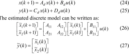
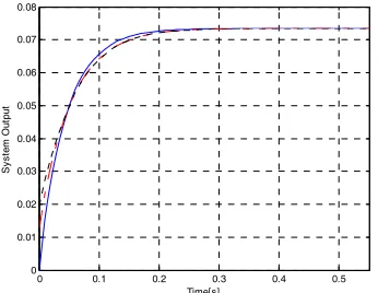
[image:6.612.332.547.528.678.2]This transformed model was simulated with an input signal that has different functions to capture most of the system dynamics as seen in Figure 4, which presents the system states while training and converging.
0 0.1 0.2 0.3 0.4 0.5 0
0.01 0.02 0.03 0.04 0.05 0.06 0.07 0.08
Time[s]
S
ys
tem
O
ut
put
It is important to notice that the eigenvalues of the original system are preserved in the transformed model as seen in the above diagonal system matrix. Reducing the 3rd order transformed model to a 2nd order model yields:
[
]
x[
]
uy
u x
x
r r
r r
0.0195
0.1856 1.0405
1.0482 0.5979 22
0
10.4534 25.2822
-+ =
⎥ ⎦ ⎤ ⎢ ⎣ ⎡ + ⎥ ⎦ ⎤ ⎢
⎣ ⎡
− =
&
with the dominant eigenvalues preserved as desired. However, by comparing this result to the result of the singular perturbation without transformation which is:
u x
xr r ⎥
⎦ ⎤ ⎢ ⎣ ⎡ + ⎥ ⎦ ⎤ ⎢
⎣ ⎡ =
1.05 0.775 29.5
-8.2
2.75 20.9
-&
[
]
x[
]
uyr=1.05 0.325 r + 0.0125
it is seen that the eigenvalues {-18.79, -31.60} are totally different from the original system eigenvalues. The three different models were tested for a step input signal and the results are shown in Figure 5.
[image:7.612.72.245.270.404.2]
Figure 5. Reduced 2nd order models (.… transformed, -.-.- transformed) output responses to a step input along with the non-reduced model ( ___ original) 3rd order system output response.
It is observed that the transformed reduced model has achieved (1) preserving the original system dominant eigenvalues and (2) performing well as compared with the original system response.
4.2 Order Model Reduction via NN and LMI-Based
System Transformation
The following example illustrates the new idea of system order model reduction using LMI with comparison to the order model reduction without using LMI.
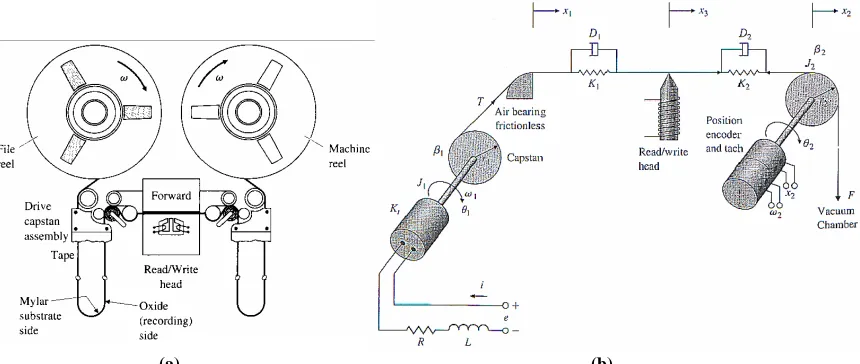
Example 2. Consider the system of a high-performance tape
transport shown in Figure 6. The system is designed with a small capstan to pull the tape past the read/write heads with the take-up reels turned by DC motors [6].
As can be shown, in static equilibrium, the tape tension equals the vacuum forceTo =F and the torque from the motor equals the torque on the capstanKtio =r1To where:
To = tape tension at the read/write head at equilibrium,
F = constant force (tape tension for vacuum column),
K = motor torque constant,
io = equilibrium motor current,
r1 = radius of the capstan take-up wheel.
The variables are defined as deviations from this equilibrium. The system motion equations are:
i K T r dt
d
J = 1+ 1 1− 1 + t
1 ω βω , x&1=r1ω1
e K Ri dt di
L + eω1= , x&2 =r2ω2
0 2 2 2 2
2ddt + +r T=
J ω β ω
) ( )
( 3 1 1 3 1
1 x x D x x
K
T = − + & −&
) ( )
( 2 3 2 2 3
2 x x D x x
K
T = − + & −&
1 1
1 rθ
x = , x2 =r2θ2, 2
2 1 3 x x
x = −
where:
D1,2 = damping in the tape-stretch motion,
e = applied input voltage V,
i = current into capstan motor,
J1 = combined inertia (wheel and take-up) motor,
J2 = inertia of the idler,
K1,2 = spring constant in the tape-stretch motion,
Ke = electric constant of the motor, Kt = torque constant of the motor, L = armature inductance,
R = armature resistance,
r1 = radius of take-up wheel,
r2 = radius of the tape on the idler,
T = tape tension at the read/write head,
x3 = position of the tape at the head,
=
3
x& velocity of the tape at the head, β1 = viscous friction at take-up wheel, β2 = viscous friction at the wheel, θ1 = angular displacement of the capstan, θ2 = tachometer shaft angle,
ω1 = speed of the drive wheelθ&1,
ω2 = output speed measured by the tachometer output θ&2. The state space form is derived from the system equations, where there is one input, which is the applied voltage, three outputs, which are: (1) tape position at the head, (2) tape tension, and (3) tape position at the wheel, and five states: (1) tape position at the air bearing, (2) drive wheel speed, (3) tape position at the wheel, (4) tachometer output speed, and (5) capstan motor speed. The following subsections present the simulation results for the investigation of different system cases using transformations with and without the use of LMI.
4.2.1 System Transformation Using Neural
Identification without LMI
This subsection presents simulations of system transformation using neural identification without LMI use.
Case #1. Consider the following case of the tape transport:
) (
1 0 0 0 0
) (
10 -0 0 0.03 -0
0 11.4 -2.4 -1.4 1.35
0 5 0 0 0
0.75 3.1 1.1 1.35 -1.1
-0 0 0 2 0
)
(t xt ut
x
⎥ ⎥ ⎥ ⎥ ⎥ ⎥
⎦ ⎤
⎢ ⎢ ⎢ ⎢ ⎢ ⎢
⎣ ⎡
+
⎥ ⎥ ⎥ ⎥ ⎥ ⎥
⎦ ⎤
⎢ ⎢ ⎢ ⎢ ⎢ ⎢
⎣ ⎡
=
0 5 10 15 20 -0.02
0 0.02 0.04 0.06 0.08 0.1 0.12 0.14
Time[s]
S
ys
tem O
ut
put
(a) (b)
Figure 6. Tape-drive system: (a) Front view of a typical tape-drive mechanism and (b) schematic control model.
) ( 0 2 . 0 2 . 0 2 . 0 2 . 0
0 0 5 . 0 0 5 . 0
0 0 1 0 0 )
(t xt
y
⎥ ⎥ ⎥
⎦ ⎤
⎢ ⎢ ⎢
⎣ ⎡
− − =
The five eigenvalues are {-10.5772, -9.999, -0.9814, -0.5962 ± j0.8702}, where two eigenvalues are complex and three are real, and thus since (1) not all the eigenvalues are complex and (2) the existing real eigenvalues produce the fast dynamics that we need to eliminate, order model reduction may be applied. As can be seen, two real eigenvalues produce fast dynamics {-10.5772, -9.999} and one real eigenvalue produces slow dynamics {-0.9814}. We performed reduction based on the estimation of the input matrix [Bˆ] and the transformed system matrix [Aˆ]. This estimation is achieved using NN.
By discretizing the above system with a sampling time Ts = 0.1 s, using a step input with learning time Tl = 300
s, training the NN for the input output data with a learning rate η = 0.005, the transformed model for [Aˆ] and [Bˆ] is:
) (
1.0107 0.0011
-0.1307 0.0974 0.1414
) (
10.5764 -0 0 0 0
0.0146 9.9985 -0 0 0
0.4680 -0.4962 0.9809 -0 0
0.3375 -0.4520 -0.8034 0.5967 -0.8701
-0.4114 -0.2710 -0.1041 -0.8701 0.5967
-)
(t xt ut
x
⎥ ⎥ ⎥ ⎥ ⎥ ⎥
⎦ ⎤
⎢ ⎢ ⎢ ⎢ ⎢ ⎢
⎣ ⎡
+
⎥ ⎥ ⎥ ⎥ ⎥ ⎥
⎦ ⎤
⎢ ⎢ ⎢ ⎢ ⎢ ⎢
⎣ ⎡
=
&
()
0 2 . 0 2 . 0 2 . 0 2 . 0
0 0 5 . 0 0 5 . 0
0 0 1 0 0 )
(t xt
y
⎥ ⎥ ⎥
⎦ ⎤
⎢ ⎢ ⎢
⎣ ⎡
− − =
As observed, all the system eigenvalues have been preserved in this transformed model with a little difference due to discretization. Using the singular perturbation technique, the following reduced 3rd order model is obtained:
) ( 0.0860 0.0652 0.1021 )
( 0.9809 -0 0
0.8034 0.5967
-0.8701
-0.1041 -0.8701 0.5967
-)
(t xt ut
x
⎥ ⎥ ⎥
⎦ ⎤
⎢ ⎢ ⎢
⎣ ⎡ + ⎥ ⎥ ⎥
⎦ ⎤
⎢ ⎢ ⎢
⎣ ⎡ =
&
) ( 0 0 0 ) ( 2 . 0 2 . 0 2 . 0
5 . 0 0 5 . 0
1 0 0 )
(t xt ut
y
⎥ ⎥ ⎥
⎦ ⎤
⎢ ⎢ ⎢
⎣ ⎡ + ⎥ ⎥ ⎥
⎦ ⎤
⎢ ⎢ ⎢
⎣ ⎡
− − =
It is also observed in the above model that the reduced order model has preserved all of its eigenvalues
{-0.9809, -0.5967 ± j0.8701} which are a subset of the original system, while the reduced order model obtained using the singular perturbation without transformation has provided different eigenvalues {-0.828, -0.598± j0.930}.
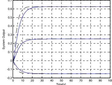
Evaluations of the reduced order models (transformed and non-transformed) were obtained by simulating both systems for a step input. Simulation results are shown in Figure 7.
[image:8.612.78.508.47.229.2]
Figure 7. Reduced 3rd order models (…. transformed, -.-.-.- transformed) output responses to a step input along with the non-reduced model ( ____ original) 5th order system output response.
Based on Figure 7, it can be seen that the non-transformed reduced order model provides a response that is better than the transformed reduced model. This is due to the transformation performed only for [A] and [B] leaving [C]
unchanged. Hence, system transformation is further considered for complete system transformation using LMI (for [A], [B], and [D]), where LMI-based transformation will
produce better reduction-based response results than both the non-transformed and transformed without LMI.
Case #2. Consider the following 2nd case:
) (
1 0 0 0 0
) (
10 -0 0 0.03 -0
0 5.4 -1.4 -0.4 0.35
0 5 0 0 0
0.75 04.1 0.1 1.35 -0.1
-0 0 0 2 0
)
(t xt ut
x
⎥ ⎥ ⎥ ⎥ ⎥ ⎥
⎦ ⎤
⎢ ⎢ ⎢ ⎢ ⎢ ⎢
⎣ ⎡
+
⎥ ⎥ ⎥ ⎥ ⎥ ⎥
⎦ ⎤
⎢ ⎢ ⎢ ⎢ ⎢ ⎢
⎣ ⎡
=
0 10 20 30 40 50 60 70 80 -0.2
-0.1 0 0.1 0.2 0.3 0.4 0.5 0.6 0.7
Time[s]
S
yst
em
O
ut
pu
t
0 1 2 3 4 5 6 7 8 -0.02
0 0.02 0.04 0.06 0.08 0.1 0.12
0.14___ Original, ---- Trans. with LMI, -.-.- None Trans., .... Trans. without LMI
Time[s]
S
ys
tem
O
ut
put
) ( 0 2 . 0 2 . 0 2 . 0 2 . 0
0 0 5 . 0 0 5 . 0
0 0 1 0 0 )
(t xt
y
⎥ ⎥ ⎥
⎦ ⎤
⎢ ⎢ ⎢
⎣ ⎡
− −
=
The eigenvalues are {-9.9973, -3.9702, -1.8992, -0.6778, -0.2055} which are all real. Utilizing the discretized model (Ts = 0.1 s) for a step input with learning time Tl = 500 s, and
training the NN for the input output data with η = 1.25 x 10⁻⁵,
and then, by applying the singular perturbation technique, the following reduced 3rd order model is obtained:
) ( 0.4649 0.0078 0.0341 ) ( 1.8986 -0 0
0.0329 -0.6782 -0
0.6966 1.5131 -0.2051 -)
(t xt ut
x
⎥ ⎥ ⎥
⎦ ⎤
⎢ ⎢ ⎢
⎣ ⎡ + ⎥ ⎥ ⎥
⎦ ⎤
⎢ ⎢ ⎢
⎣ ⎡ =
&
) ( 0017 . 0
0 0 ) ( 2 . 0 2 . 0 2 . 0
5 . 0 0 5 . 0
1 0 0 )
(t xt ut
y
⎥ ⎥ ⎥
⎦ ⎤
⎢ ⎢ ⎢
⎣ ⎡ + ⎥ ⎥ ⎥
⎦ ⎤
⎢ ⎢ ⎢
⎣ ⎡
− − =
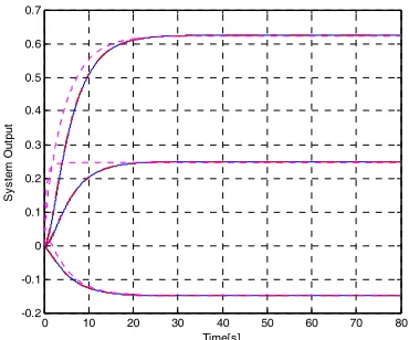
Again, it is seen here the preservation of the reduced order model eigenvalues being as a subset of the original system. However, as shown before, the reduced order model without system transformation provided different eigenvalues {-1.5165, -0.6223, -0.2060} from the transformed reduced order model. Simulating both systems for a step input provided the results shown in Figure 8.
[image:9.612.73.258.320.474.2]
Figure 8. Reduced 3rd order models (…. transformed, -.-.-.- transformed) output responses to a step input along with the non-reduced ( ____ original) 5th order system output response.
In Figure 8, it is also seen that the response of the non-transformed reduced order model is better than the transformed reduced model, which is again caused by leaving the output [C] matrix without transformation.
4.2.2 LMI-Based State Transformation via Neural
Identification
As previously observed, the system transformation without using LMI, where its objective was to preserve the system eigenvalues in the reduced order model, did not provide an accurate response as compared with either the reduced non-transformed or the original responses. As was explained, this was due to the fact of not transforming the complete system (i.e., by neglecting the [C] matrix). In order to achieve better
response, we will now perform a complete system transformation using LMI to obtain the permutation matrix
[P]. The following presents simulations for the previously
considered tape drive system cases.
Case #1. For the example of case #1 in subsection 4.2.1, the
NN estimation is used now to estimate only the transformed [Ad
~
] matrix. Discretizing the system with Ts = 0.1 s, using a
step input with learning time Tl = 15 s, and training the NN
for the input output data with η = 0.001, produces the transformed system matrix:
⎥ ⎥ ⎥ ⎥ ⎥ ⎥
⎦ ⎤
⎢ ⎢ ⎢ ⎢ ⎢ ⎢
⎣ ⎡
=
10.5764 -0 0 0 0
1.0449 9.9985 -0 0 0
0.4934 0.1395 0.9809 -0 0
0.2114 0.6165 0.2276 0.5967 -0.8701
-0.0964 0.9860 -1.4633 -0.8701 0.5967
-~
A
Based on this transformed matrix, using LMI, the permutation matrix [P] was computed and then used for the
complete system transformation. Thus, the transformed {[B~], [C~], [D~]} matrices were then obtained. Performing
order model reduction provided the 3rd order reduced model: ) ( 4.1652
-47.3374
-35.1670 )
( 0.9809 -0 0
0.2276 0.5967 -0.8701
-1.4633 -0.8701 0.5967 -)
(t xt ut
x
⎥ ⎥ ⎥
⎦ ⎤
⎢ ⎢ ⎢
⎣ ⎡ + ⎥ ⎥ ⎥
⎦ ⎤
⎢ ⎢ ⎢
⎣ ⎡ =
&
) ( 0.0006
0.0025 -
0.0025 -) ( 0.0021 -0.0004 0.0001
-0.0088 -0.0009 -0.0024
-0.0139 -0 0.0019 -)
(t xt ut
y
⎥ ⎥ ⎥
⎦ ⎤
⎢ ⎢ ⎢
⎣ ⎡ + ⎥ ⎥ ⎥
⎦ ⎤
⎢ ⎢ ⎢
⎣ ⎡ =
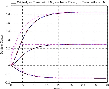
where the objective of eigenvalue preservation is clearly achieved. Investigating the performance of this new LMI-based reduced order model shows clearly that the new completely transformed system is better than all of the previous reduced models. This is shown in Figure 9. As seen in the figure, the 3rd order reduced model, based on LMI transformation, provided a response that is almost the same as the 5th order original system response.
Figure 9. Reduced 3rd order models (…. transformed without LMI, .-.-.- non-transformed, ---- transformed with LMI) output responses to a step input along with the non reduced ( ____ original) system output response. The LMI-transformed curve fits almost exactly on the original response.
Case #2. Investigating the example of case #2 in subsection
4.2.1, for Ts = 0.1 s, 200 input/output data points, and
η = 1 x 10⁻⁴, the LMI-based transformation and then order
[image:9.612.325.520.442.596.2]0 5 10 15 20 25 30 35 40 -0.2
-0.1 0 0.1 0.2 0.3 0.4 0.5 0.6
0.7___ Original, ---- Trans. with LMI, -.-.- None Trans., .... Trans. without LMI
Time[s]
S
ys
tem
Ou
tp
ut
0 1 2 3 4 5 6 7 8 9 10
0 0.02 0.04 0.06 0.08 0.1 0.12
0.14 Step Response
Time (sec)
A
m
pl
[image:10.612.65.257.57.214.2]itude
Figure 10. Reduced 3rd order models (…. transformed without LMI, -.-.-.- non-transformed, ---- transformed with LMI) output responses to a step input along with the non reduced ( ____ original) system output response. The LMI-transformed curve fits almost exactly on the original response.
Again, the response of the reduced order model using the complete LMI-based transformation is the best as compared to the other reduction techniques.
5. CLOSED LOOP FEEDBACK CONTROL FOR THE REDUCED ORDER MODELS
Using the LMI-based reduced system models presented in the previous section, different control techniques are considered in this section to obtain the desired system performance.
5.1 PID Control
A PID controller is a control feedback method which is widely used in industrial control systems [4,6]. It attempts to correct the error between a measured process variable (output) and a desired set-point (input) by calculating and then providing a corrective signal that can adjust the process as shown in Figure 11.
Figure 11. Single-input single-output (SISO) closed-loop feedback control using a PID controller.
In the control design process, the three parameters of the PID controller {Kp, Ki, Kd} have to be calculated for
some specific process requirements such as system overshoot and settling time. It is normal that once they are calculated and implemented, the response of the system is not actually as desired. Therefore, further tuning of these parameters is needed to provide the desired control action.
For the system of LMI-based case #1, focusing on one output of the tape-drive machine, we investigated the
PID controller using the reduced order model for the desired output that we are interested in. Thus, the estimated reduced 3rd order model is now considered for the output of the tape position at the head represented by:
1.0919 2.2837s
2.1742s
0.133 0.0801s )
( original 3 2
+ +
+
+ =
s s
G
Searching for suitable values of the PID controller parameters, such that the system provides a faster response settling time and less overshoot, it is found that Kp = 100, Ki = 80, and Kd = 90 with a controlled system given by:
10.64 20.8s 22.26s
9.383 s
10.64 19.71s 19.98s
7.209s )
( controlled 4 3 3 2 2
+ + +
+
+ +
+ =
s s
G
Simulating the PID controlled system for a step input shows the results in Figure 12, where the settling time is 1.5 s while without the controller was 6.5 s. Also as observed, the overshoot has much decreased after using the PID controller.
Figure 12. Reduced 3rd order model PID controlled and uncontrolled step responses.
On the other hand, the other system outputs can be PID-controlled using the cascading of current process PID and new tuning-based PIDs for each output. For the PID-controlled output of the tachometer shaft angle, the controlling scheme would be as shown in Figure 13.
Figure 13. Single-input multiple-output (SIMO) closed loop feedback system with a PID controller.
As seen in Figure 13, the output of interest (2nd output) is controlled as desired using the PID controller. However, this will affect the other outputs performance and therefore a further PID-based tuning operation must be applied. As shown in Figure 13, the tuning process is accomplished using G1T and G3T. For example, for the 1st
output G1:
R G Y Y R G G
[image:10.612.326.541.251.414.2] [image:10.612.75.276.481.572.2] [image:10.612.327.532.497.581.2]0 10 20 30 40 50 60 70 80 90 100 -0.2
-0.1 0 0.1 0.2 0.3 0.4 0.5 0.6 0.7
Time[s]
S
ys
te
m
O
ut
put
0 10 20 30 40 50 60 70 80 90 100 -0.2
-0.1 0 0.1 0.2 0.3 0.4 0.5 0.6 0.7
Time[s]
S
ys
tem
O
ut
put
or
B +
+
+
y(t)
u(t)
) ( ~x t
r
& ~xr(t)
K
- +
r(t)
or
A
or C or D
+
∫
∴
) PID( 2
1 RR-Y
GT = (40) where Y2 is the Laplace transform of the 2nd output. Similarly,
G3T can be obtained for the 3rd output G3.
5.2 State Feedback Control
In this section, we will present the state feedback control (SFC) using pole placement and the LQR optimal control.
5.2.1 SFC via Pole Placement
For the reduced order model in the system of Equations (37) and (38), an LQR-based state feedback controller can be designed. For example, assuming that a controller is needed to provide the system with an enhanced system performance by relocating the eigenvalues, this objective can be achieved using the control input given by:
) ( ) ( ~ )
(t Kx t rt
u =− r + (41)
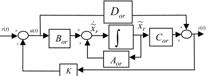
[image:11.612.329.510.50.190.2]where K is the state feedback gain designed based on the desired system eigenvalues. A state feedback control for pole placement can be illustrated as shown in Figure 14.
Figure 14. Block diagram of a state feedback control (SFC) with {[Aor], [Bor], [Cor], [Dor]} overall reduced order system
matrices.
Replacing the control input u(t) in Equations (37) and (38) by the above new control input in Equation (41) gives the following reduced system equations:
)] ( ) ( ~ [ ) ( ~ ) (
~x t A x t B Kx t r t
r or r
or
r = + − +
& (42)
)] ( ) ( ~ [ ) ( ~ )
(t C x t D Kx t r t
y = or r + or − r + (43) which can be re-written as:
) ( ) ( ~ )
( ~ ) (
~x t A x t B Kx t B r t
or r or r or
r = − +
&
=[Aor −BorK]x~r(t)+Borr(t) ) ( ) ( ~ )
( ~ )
(t C x t D Kx t D r t
y = or r − or r + or
=[Cor −DorK]x~r(t)+Dorr(t)
The overall closed-loop system model can be written as: )
( ) ( ~ ) (
~x t A x t B r t
cl r
cl +
=
& (44) )
( ) ( ~ )
(t C x t D rt
y = cl r + cl (45)
such that the closed loop system matrix [Acl] will provide the
new desired system eigenvalues.
[image:11.612.55.293.306.401.2]For example, for the system of case #2 using LMI, the state feedback was used to replace the eigenvalues by {-1.89, -1.5, -1}. The feedback control was found K = [-1.2098 0.3507 0.0184], which placed the eigenvalues as desired and enhanced the system performance as observed in Figure 15.
Figure 15. Reduced 3rd order state feedback control (for pole placement) output step response .-.-.- compared with the original ____ full order system output step response.
5.2.2 SFC via LQR Optimal Control
Another method for designing SFC may be achieved by minimizing the cost function given by [6]:
(
)
∫
∞
+ =
0
dt Ru u Qx x
J T T (46) which is defined for the system x&(t)=Ax(t)+Bu(t), where
Q and R are weight matrices for the system states and inputs. This is known as the LQR problem, [4,6]. The feedback control law that minimizes the values of the cost is given by:
) ( )
(t Kxt
u =− (47) where K is the solution of K=R−1BTq and [q] is found by
solving the algebraic Riccati equation described by: 0
1 + =
−
+qA qBR− B q Q
q
AT T (48) A direct solution for the optimal control gain maybe obtained using the MATLAB statement K=lqr(A,B,Q,R), where in our example R = 1, and Q=CTC.
The LQR optimization is applied to the reduced 3rd order model in case #2 of subsection 4.2.2. The state feedback optimal control gain K = [-0.0967 -0.0192 0.0027], which when simulating the complete system for a step input, provided the normalized output response (with a normalization factor γ = 1.934) as shown in Figure 16.
[image:11.612.336.520.550.689.2]