Lewis, F.L.; et. al.
“
Robotics
”
Mechanical Engineering Handbook
Ed.
Frank Kreith
Boca Raton: CRC Press LLC,
1999
c
Robotics
14.1 Introduction ...14-2 14.2 Commercial Robot Manipulators...14-3
Commercial Robot Manipulators • Commercial Robot Controllers
14.3 Robot Configurations ...14-15
Fundamentals and Design Issues • Manipulator Kinematics • Summary
14.4 End Effectors and Tooling ...14-24
A Taxonomy of Common End Effectors • End Effector Design Issues • Summary
14.5 Sensors and Actuators ...14-33
Tactile and Proximity Sensors • Force Sensors • Vision • Actuators
14.6 Robot Programming Languages ...14-48
Robot Control • System Control • Structures and Logic • Special Functions • Program Execution • Example Program • Off-Line Programming and Simulation
14.7 Robot Dynamics and Control ...14-51
Robot Dynamics and Properties • State Variable Representations and Computer Simulation • Cartesian Dynamics and Actuator Dynamics • Computed-Torque (CT) Control and Feedback Linearization • Adaptive and Robust Control • Learning Control • Control of Flexible-Link and Flexible-Joint Robots • Force Control • Teleoperation
14.8 Planning and Intelligent Control...14-69
Path Planning • Error Detection and Recovery • Two-Arm Coordination • Workcell Control • Planning and Artifical Intelligence • Man-Machine Interface
14.9 Design of Robotic Systems...14-77
Workcell Design and Layout • Part-Feeding and Transfers
14.10 Robot Manufacturing Applications...14-84
Product Design for Robot Automation • Economic Analysis • Assembly
14.11 Industrial Material Handling and Process Applications of Robots...14-90
Implementation of Manufacturing Process Robots • Industrial Applications of Process Robots
14.12 Mobile, Flexible-Link, and Parallel-Link Robots ...14-102
Mobile Robots • Flexible-Link Robot Manipulators • Parallel-Link Robots
Frank L. Lewis
University of Texas at Arlington
John M. Fitzgerald
University of Texas at Arlington
Ian D. Walker
Rice University
Mark R. Cutkosky
Stanford University
Kok-Meng Lee
Georgia Tech
Ron Bailey
University of Texas at Arlington
Frank L. Lewis
University of Texas at Arlington
Chen Zhou
Georgia Tech
John W. Priest
University of Texas at Arlington
G. T. Stevens, Jr.
University of Texas at Arlington
John M. Fitzgerald
University of Texas at Arlington
Kai Liu
14-2 Section 14
14.1 Introduction
The word “robot” was introduced by the Czech playright Karel ˇCapek in his 1920 play Rossum’s Universal Robots. The word “robota” in Czech means simply “work.” In spite of such practical begin-nings, science fiction writers and early Hollywood movies have given us a romantic notion of robots. Thus, in the 1960s robots held out great promises for miraculously revolutionizing industry overnight. In fact, many of the more far-fetched expectations from robots have failed to materialize. For instance, in underwater assembly and oil mining, teleoperated robots are very difficult to manipulate and have largely been replaced or augmented by “smart” quick-fit couplings that simplify the assembly task. However, through good design practices and painstaking attention to detail, engineers have succeeded in applying robotic systems to a wide variety of industrial and manufacturing situations where the environment is structured or predictable. Today, through developments in computers and artificial intel-ligence techniques and often motivated by the space program, we are on the verge of another breakthrough in robotics that will afford some levels of autonomy in unstructured environments.
On a practical level, robots are distinguished from other electromechanical motion equipment by their dexterous manipulation capability in that robots can work, position, and move tools and other objects with far greater dexterity than other machines found in the factory. Process robot systems are functional components with grippers, end effectors, sensors, and process equipment organized to perform a con-trolled sequence of tasks to execute a process — they require sophisticated control systems.
The first successful commercial implementation of process robotics was in the U.S. automobile industry. The word “automation” was coined in the 1940s at Ford Motor Company, as a contraction of “automatic motivation.” By 1985 thousands of spot welding, machine loading, and material handling applications were working reliably. It is no longer possible to mass produce automobiles while meeting currently accepted quality and cost levels without using robots. By the beginning of 1995 there were over 25,000 robots in use in the U.S. automobile industry. More are applied to spot welding than any other process. For all applications and industries, the world’s stock of robots is expected to exceed 1,000,000 units by 1999.
The single most important factor in robot technology development to date has been the use of microprocessor-based control. By 1975 microprocessor controllers for robots made programming and executing coordinated motion of complex multiple degrees-of-freedom (DOF) robots practical and reliable. The robot industry experienced rapid growth and humans were replaced in several manufacturing processes requiring tool and/or workpiece manipulation. As a result the immediate and cumulative dangers of exposure of workers to manipulation-related hazards once accepted as necessary costs have been removed.
A distinguishing feature of robotics is its multidisciplinary nature — to successfully design robotic systems one must have a grasp of electrical, mechanical, industrial, and computer engineering, as well as economics and business practices. The purpose of this chapter is to provide a background in all these areas so that design for robotic applications may be confronted from a position of insight and confidence. The material covered here falls into two broad areas: function and analysis of the single robot, and design and analysis of robot-based systems and workcells.
Robotics 14-3
14.2 Commercial Robot Manipulators
John M. Fitzgerald
In the most active segments of the robot market, some end-users now buy robots in such large quantities (occasionally a single customer will order hundreds of robots at a time) that market prices are determined primarily by configuration and size category, not by brand. The robot has in this way become like an economic commodity. In just 30 years, the core industrial robotics industry has reached an important level of maturity, which is evidenced by consolidation and recent growth of robot companies. Robots are highly reliable, dependable, and technologically advanced factory equipment. There is a sound body of practical knowledge derived from a large and successful installed base. A strong foundation of theoretical robotics engineering knowledge promises to support continued technical growth.
The majority of the world’s robots are supplied by established stable companies using well-established off-the-shelf component technologies. All commercial industrial robots have two physically separate basic elements: the manipulator arm and the controller. The basic architecture of all commercial robots is fundamentally the same. Among the major suppliers the vast majority of industrial robots uses digital servo-controlled electrical motor drives. All are serial link kinematic machines with no more than six axes (degrees of freedom). All are supplied with a proprietary controller. Virtually all robot applications require significant effort of trained skilled engineers and technicians to design and implement them. What makes each robot unique is how the components are put together to achieve performance that yields a competitive product. Clever design refinements compete for applications by pushing existing performance envelopes, or sometimes creating new ones. The most important considerations in the application of an industrial robot center on two issues: Manipulation and Integration.
Commercial Robot Manipulators
Manipulator Performance CharacteristicsThe combined effects of kinematic structure, axis drive mechanism design, and real-time motion control determine the major manipulation performance characteristics: reach and dexterity, payload, quickness, and precision. Caution must be used when making decisions and comparisons based on manufacturers’ published performance specifications because the methods for measuring and reporting them are not standardized across the industry. Published performance specifications provide a reasonable comparison of robots of similar kinematic configuration and size, but more detailed analysis and testing will insure that a particular robot model can reach all of the poses and make all of the moves with the required payload and precision for a specific application.
Reach is characterized by measuring the extents of the space described by the robot motion and dexterity by the angular displacement of the individual joints. Horizontal reach, measured radially out from the center of rotation of the base axis to the furthest point of reach in the horizontal plane, is usually specified in robot technical descriptions. For Cartesian robots the range of motion of the first three axes describes the reachable workspace. Some robots will have unusable spaces such as dead zones, singular poses, and wrist-wrap poses inside of the boundaries of their reach. Usually motion test, simulations, or other analysis are used to verify reach and dexterity for each application.
Payload weight is specified by the manufacturer for all industrial robots. Some manufacturers also specify inertial loading for rotational wrist axes. It is common for the payload to be given for extreme velocity and reach conditions. Load limits should be verified for each application, since many robots can lift and move larger-than-specified loads if reach and speed are reduced. Weight and inertia of all tooling, workpieces, cables, and hoses must be included as part of the payload.
14-4 Section 14
characteristic of interest. Some manufacturers give cycle times for well-described motion cycles. These motion profiles give a much better representation of quickness. Most robot manufacturers address the issue by conducting application-specific feasibility tests for customer applications.
Precision is usually characterized by measuring repeatability. Virtually all robot manufacturers specify static position repeatability. Usually, tool point repeatability is given, but occasionally repeatability will be quoted for each individual axis. Accuracy is rarely specified, but it is likely to be at least four times larger than repeatability. Dynamic precision, or the repeatability and accuracy in tracking position, velocity, and acceleration on a continuous path, is not usually specified.
Common Kinematic Configurations
All common commercial industrial robots are serial link manipulators with no more than six kinemat-ically coupled axes of motion. By convention, the axes of motion are numbered in sequence as they are encountered from the base on out to the wrist. The first three axes account for the spatial positioning motion of the robot; their configuration determines the shape of the space through which the robot can be positioned. Any subsequent axes in the kinematic chain provide rotational motions to orient the end of the robot arm and are referred to as wrist axes. There are, in principle, two primary types of motion that a robot axis can produce in its driven link: either revoluteor prismatic. It is often useful to classify robots according to the orientation and type of their first three axes. There are four very common commercial robot configurations: Articulated, Type 1 SCARA, Type 2 SCARA, and Cartesian. Two other configurations, Cylindrical and Spherical, are now much less common.
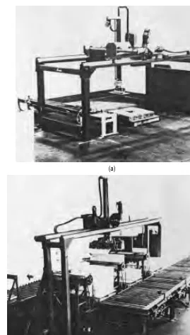
Articulated Arms. The variety of commercial articulated arms, most of which have six axes, is very large. All of these robots’ axes are revolute. The second and third axes are parallel and work together to produce motion in a vertical plane. The first axis in the base is vertical and revolves the arm sweeping out a large work volume. The need for improved reach, quickness, and payload have continually motivated refinements and improvements of articulated arm designs for decades. Many different types of drive mechanisms have been devised to allow wrist and forearm drive motors and gearboxes to be mounted close in to the first and second axis rotation to minimize the extended mass of the arm. Arm structural designs have been refined to maximize stiffness and strength while reducing weight and inertia. Special designs have been developed to match the performance requirements of nearly all industrial applications and processes. The workspace efficiency of well-designed articulated arms, which is the degree of quick dexterous reach with respect to arm size, is unsurpassed by other arm configurations when five or more degrees of freedom are needed. Some have wide ranges of angular displacement for both the second and third axis, expanding the amount of overhead workspace and allowing the arm to reach behind itself without making a 180° base rotation. Some can be inverted and mounted overhead on moving gantries for transportation over large work areas. A major limiting factor in articulated arm performance is that the second axis has to work to lift both the subsequent arm structure and payload. Springs, pneumatic struts, and counterweights are often used to extend useful reach. Historically, articulated arms have not been capable of achieving accuracy as well as other arm configurations. All axes have joint angle position errors which are multiplied by link radius and accumulated for the entire arm. However, new articulated arm designs continue to demonstrate improved repeatability, and with practical calibration methods they can yield accuracy within two to three times the repeatability. An example of extreme precision in articulated arms is the Staubli Unimation RX arm (see Figure 14.2.1).
Robotics 14-5
(a)
(b)
14-6 Section 14
(c)
(d)
Robotics 14-7
well-known optimal SCARA design is the AdeptOne robot shown in Figure 14.2.2a. It can move a 20-lb payload from point “A” up 1 in. over 12 in. and down 1 in. to point “B” and return through the same path back to point “A” in less than 0.8 sec (see Figure 14.2.2).
Type II SCARA. The Type 2 SCARA, also a four-axis configuration, differs from Type 1 in that the first axis is a long, vertical, prismatic Z stroke which lifts the two parallel revolute axes and their links. For quickly moving heavier loads (over approximately 75 lb) over longer distances (over about 3 ft), the Type 2 SCARA configuration is more efficient than the Type 1. The trade-off of weight vs. inertia vs. quickness favors placement of the massive vertical lift mechanism at the base. This configuration is well suited to large mechanical assembly and is most frequently applied to palletizing, packaging, and other heavy material handling applications (see Figure 14.2.3).
Cartesian Coordinate Robots. Cartesian coordinate robots use orthogonal prismatic axes, usually referred to as X, Y, and Z, to translate their end-effector or payload through their rectangular workspace. One, two, or three revolute wrist axes may be added for orientation. Commercial robot companies supply several types of Cartesian coordinate robots with workspace sizes ranging from a few cubic inches to tens of thousands of cubic feet, and payloads ranging to several hundred pounds. Gantry robots are the most common Cartesian style. They have an elevated bridge structure which translates in one horizontal direction on a pair of runway bearings (usually referred to as the X direction), and a carriage which
(a)
14-8 Section 14
moves along the bridge in the horizontal “Y” direction also usually on linear bearings. The third orthogonal axis, which moves in the Z direction, is suspended from the carriage. More than one robot can be operated on a gantry structure by using multiple bridges and carriages. Gantry robots are usually supplied as semicustom designs in size ranges rather than set sizes. Gantry robots have the unique capacity for huge accurate work spaces through the use of rigid structures, precision drives, and work-space calibration. They are well suited to material handling applications where large areas and/or large loads must be serviced. As process robots they are particularly useful in applications such as arc welding, waterjet cutting, and inspection of large, complex, precision parts.
Modular Cartesian robots are also commonly available from several commercial sources. Each module is a self-contained completely functional single axis actuator. Standard liner axis modules which contain all the drive and feedback mechanisms in one complete structural/functional element are coupled to perform coordinated three-axis motion. These modular Cartesian robots have work volumes usually on the order of 10 to 30 in. in X and Y with shorter Z strokes, and payloads under 40 lb. They are typically used in many electronic and small mechanical assembly applications where lower performance than Type 1 SCARA robots is suitable (see Figure 14.2.4).
Spherical and Cylindrical Coordinate Robots. The first two axes of the spherical coordinate robot are revolute and orthogonal to one another, and the third axis provides prismatic radial extension. The result is a natural spherical coordinate system and a work volume that is spherical. The first axis of cylindrical coordinate robots is a revolute base rotation. The second and third are prismatic, resulting in a natural cylindrical motion.
(b)
Robotics 14-9
Commerical models of spherical and cylindrical robots were originally very common and popular in machine tending and material handling applications. Hundreds are still in use but now there are only a few commercially available models. The Unimate model 2000, a hydraulic-powered spherical coordinate robot, was at one time the most popular robot model in the world. Several models of cylindrical coordinate robots were also available, including a standard model with the largest payload of any robot, the Prab model FC, with a payload of over 600 kg. The decline in use of these two configuations is attributed to problems arising from use of the prismatic link for radial extension/retraction motion. A solid boom requires clearance to fully retract. Hydraulic cylinders used for the same function can retract to less than half of their fully extended length. Type 2 SCARA arms and other revolute jointed arms have displaced most of the cylindrical and spherical coordinate robots (see Figure 14.2.5).
Basic Performance Specifications. Figure 14.2.6 sumarizes the kinematic configurations just described.
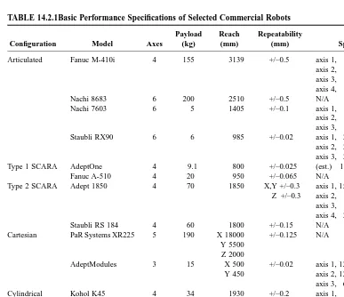
[image:10.612.136.370.68.393.2]Table 14.2.1 is a table of basic performance specifications of selected robot models that illustrates the broad spectrum of manipulator performance available from commercial sources. The information con-tained in the table has been supplied by the respective robot manufacturers. This is not an endorsement by the author or publisher of the robot brands selected, nor is it a verification or validation of the performance values. For more detailed and specific information on the availability of robots, the reader is advised to contact the Robotic Industries Association, 900 Victors Way, P.O. Box 3724, Ann Arbor, MI 48106, or a robot industry trade association in your country for a listing of commercial robot suppliers and system integrators.
14-10 Section 14
Drive Types of Commerical Robots
The vast majority of commerical industrial robots uses electric servo motor drives with speed-reducting transmissions. Both AC and DC motors are popular. Some servo hydraulic articulated arm robots are available now for painting applications. It is rare to find robots with servo pneumatic drive axes. All types of mechanical transmissions are used, but the tendency is toward low and zero backlash-type drives. Some robots use direct drive methods to eliminate the amplification of inertia and mechanical backlash associated with other drives. The first axis of the AdeptOne and AdeptThree Type I SCARA
(a)
[image:11.612.119.388.69.542.2](b)
Robotics 14-11
[image:12.612.65.441.79.460.2](c)
FIGURE 14.2.4 continued
(a) (b)
14-12 Section 14
FIGURE 14.2.6 Common kinematic configurations for robots.
TABLE 14.2.1Basic Performance Specifications of Selected Commercial Robots
Configuration Model Axes
Payload (kg)
Reach (mm)
Repeatability
(mm) Speed
Articulated Fanuc M-410i 4 155 3139 +/–0.5 axis 1, 85 deg/sec axis 2, 90 deg/sec axis 3, 100 deg/sec axis 4, 190 deg/sec Nachi 8683 6 200 2510 +/–0.5 N/A
Nachi 7603 6 5 1405 +/–0.1 axis 1, 115 deg/sec axis 2, 115 deg/sec axis 3, 115 deg/sec Staubli RX90 6 6 985 +/–0.02 axis 1, 240 deg/sec axis 2, 200 deg/sec axis 3, 286 deg/sec Type 1 SCARA AdeptOne 4 9.1 800 +/–0.025 (est.) 1700 mm/sec
Fanuc A-510 4 20 950 +/–0.065 N/A Type 2 SCARA Adept 1850 4 70 1850 X,Y +/–0.3
Z +/–0.3
axis 1, 1500 mm/sec axis 2, 120 deg/sec axis 3, 140 deg/sec axis 4, 225 deg/sec Staubli RS 184 4 60 1800 +/–0.15 N/A
Cartesian PaR Systems XR225 5 190 X 18000 Y 5500 Z 2000
+/–0.125 N/A
AdeptModules 3 15 X 500 Y 450
+/–0.02 axis 1, 1200 mm/sec axis 2, 1200 mm/sec axis 3, 600 mm/sec Cylindrical Kohol K45 4 34 1930 +/–0.2 axis 1, 90 deg/sec axis 2, 500 mm/sec axis 3, 1000 mm/sec Spherical Unimation 2000
(Hydraulic, not in production)
Robotics 14-13
robots is a direct drive motor with the motor stator integrated into the robot base and its armature rotor integral with the first link. Other more common speed-reducing low backlash drive transmissions include toothed belts, roller chains, roller drives, and harmonic drives.
Joint angle position and velocity feedback devices are generally considered an important part of the drive axis. Real-time control performance for tracking position and velocity commands and precision is often affected by the fidelity of feedback. Resolution, signal-to-noise, and innate sampling frequency are important motion control factors ultimately limited by the type of feedback device used.
Given a good robot design, the quality of fabrication and assembly of the drive components must be high to yield good performance. Because of their precision requirements, the drive components are sensitive to manufacturing errors which can readily translate to less than specified manipulator perfor-mance.
Commercial Robot Controllers
Commercial robot controllers are specialized multiprocessor computing systems that provide four basic processes allowing integration of the robot into an automation system. These functions which must be factored and weighed for each specific application are Motion Generation, Motion/Process Integration, Human Integration, and Information Integration.
Motion Generation
There are two important controller-related aspects of industrial robot motion generation. One is the extent of manipulation that can be programmed; the other is the ability to execute controlled programmed motion. The unique aspect of each robot system is its real-time kinematic motion control. The details of real-time control are typically not revealed to the user due to safety and proprietary information secrecy reasons. Each robot controller, through its operating system programs, converts digital data into coordinated motion through precise coordination and high speed distribution and communication of the individual axis motion commands which are executed by individual joint controllers. The higher level programming accessed by the end user is a reflection of the sophistication of the real-time controller.
Of greatest importance to the robot user is the motion programming. Each robot manufacturer has its own proprietary programming language. The variety of motion and position command types in a programming language is usually a good indication of the robot’s motion generation capability. Program commands which produce complex motion should be available to support the manipulation needs of the application. If palletizing is the application, then simple methods of creating position commands for arrays of positions are essential. If continuous path motion is needed, an associated set of continuous motion commands should be available. The range of motion generation capabilities of commercial industrial robots is wide. Suitability for a particular application can be determined by writing test code.
Motion/Process Integration
14-14 Section 14
reasons are that data communication is much more efficient due to data bus access, and computing operations are coordinated by one operating system.
Human Integration
Operator integration is critical to the expeditious setup, programming, and maintenance of the robot system. Three controller elements most important for effective human integration are the human I/O devices, the information available to the operator in graphic form, and the modes of operation available for human interaction. Position and path teaching effort is dramatically influenced by the type of manual I/O devices available. A teach pendant is needed if the teacher must have access to several vantage points for posing the robot. Some robots have teleoperator-style input devices which allow coordinated manual motion command inputs. These are extremely useful for teaching multiple complex poses. Graphical interfaces, available on some industrial robots, are very effective for conveying information to the operator quickly and efficiently. A graphical interface is most important for applications which require frequent reprogramming and setup changes. Several very useful off-line programming software systems are available from third-party suppliers. These systems use computer models of commercially available robots to simulate path motion and provide rapid programming functions.
Information Integration
Robotics 14-15
14.3 Robot Configurations
Ian D. Walker
Fundamentals and Design Issues
A robot manipulator is fundamentally a collection of links connected to each other by joints, typically with an end effector (designed to contact the environment in some useful fashion) connected to the mechanism. A typical arrangement is to have the links connected serially by the joints in an open-chain fashion. Each joint provides one or more degree of freedom to the mechanism.
Manipulator designs are typically characterized by the number of independent degrees of freedom in the mechanism, the types of joints providing the degrees of freedom, and the geometry of the links connecting the joints. The degrees of freedom can be revolute (relative rotational motion θ between joints) or prismatic (relative linear motion d between joints). A joint may have more than one degree of freedom. Most industrial robots have a total of six independent degrees of freedom. In addition, most current robots have essentially rigid links (we will focus on rigid-link robots throughout this section).
Robots are also characterized by the type of actuators employed. Typically manipulators have hydraulic or electric actuation. In some cases where high precision is not important, pneumatic actuators are used. A number of successful manipulator designs have emerged, each with a different arrangement of joints and links. Some “elbow” designs, such as the PUMA robots and the SPAR Remote Manipulator System, have a fairly anthropomorphic structure, with revolute joints arranged into “shoulder,” “elbow,” and “wrist” sections. A mix of revolute and prismatic joints has been adopted in the Stanford Manipulator and the SCARA types of arms. Other arms, such as those produced by IBM, feature prismatic joints for the “shoulder,” with a spherical wrist attached. In this case, the prismatic joints are essentially used as positioning devices, with the wrist used for fine motions.
The above designs have six or fewer degrees of freedom. More recent manipulators, such as those of the Robotics Research Corporation series of arms, feature seven or more degrees of freedom. These arms are termed kinematically redundant, which is a useful feature as we will see later.
Key factors that influence the design of a manipulator are the tractability of its geometric (kinematic) analysis and the size and location of its workspace. The workspace of a manipulator can be defined as the set of points that are reachable by the manipulator (with fixed base). Both shape and total volume are important. Manipulator designs such as the SCARA are useful for manufacturing since they have a simple semicylindrical connected volume for their workspace (Spong and Vidyasagar, 1989), which facilitates workcell design. Elbow manipulators tend to have a wider volume of workspace, however the workspace is often more difficult to characterize. The kinematic design of a manipulator can tailor the workspace to some extent to the operational requirements of the robot.
In addition, if a manipulator can be designed so that it has a simplified kinematic analysis, many planning and control functions will in turn be greatly simplified. For example, robots with spherical wrists tend to have much simpler inverse kinematics than those without this feature. Simplification of the kinematic analysis required for a robot can significantly enhance the real-time motion planning and control performance of the robot system. For the rest of this section, we will concentrate on the kinematics of manipulators.
14-16 Section 14
Manipulator Kinematics
The study of manipulator kinematics at the position (geometric) level separates naturally into two subproblems: (1) finding the position/orientation of the end effector, or task, frame, given the angles and/or displacements of the joints (Forward Kinematics); and (2) finding possible angles/displacements of the joints given the position/orientation of the end effector, or task, frame (Inverse Kinematics). At the velocity level, the Manipulator Jacobian relates joint velocities to end effector velocities and is important in motion planning and for identifying Singularities. In the case of Redundant Manipulators, the Jacobian is particularly crucial in planning and controlling robot motions. We will explore each of these issues in turn in the following subsections.
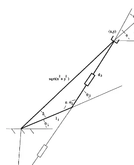
[image:17.612.189.315.291.459.2]Example 14.3.1
Figure 14.3.1 shows a planar three-degrees-of-freedom manipulator. The first two joints are revolute, and the third is prismatic. The end effector position (x, y) is expressed with respect to the (fixed) world coordinate frame (x0, y0), and the orientation of the end effector is defined as the angle of the second
link φ measured from the x0 axis as shown. The link length l1 is constant. The joint variables are given
by the angles θ1 and θ2 and the displacement d3, and are defined as shown. The example will be used
throughout this section to demonstrate the ideas behind the various kinematic problems of interest.
Forward (Direct) Kinematics
Since robots typically have sensors at their joints, making available measurements of the joint configu-rations, and we are interested in performing tasks at the robot end effector, a natural issue is that of determining the end effector position/orientation Y given a joint configuration q. This problem is the forward kinematics problem and may be expressed symbolically as
(14.3.1) The forward kinematic problem yields a unique solution for Y given q. In some simple cases (such as the example below) the forward kinematics can be derived by inspection. In general, however, the relationship f can be quite complex. A systematic method for determining the function f for any manipulator geometry was proposed by Denavit and Hartenberg (Denavit and Hartenberg, 1955).
The Denavit/Hartenberg (or D-H) technique has become the standard method in robotics for describing the forward kinematics of a manipulator. Essentially, by careful placement of a series of coordinate
FIGURE 14.3.1 Planar RRP manipulator.
frames fixed in each link, the D-H technique reduces the forward kinematics problem to that of combining a series of straightforward consecutive link-to-link transformations from the base to the end effector frame. Using this method, the forward kinematics for any manipulator is summarized in a table of parameters (the D-H parameters). A maximum of three nonzero parameters per link are sufficient to uniquely specify the map f. Lack of space prevents us from detailing the method further. The interested reader is referred to Denavit and Hartenberg (1955) and Spong and Vidyasagar (1989).
To summarize, forward kinematics is an extremely important problem in robotics which is also well understood, and for which there is a standard solution technique
Example 14.3.2
In our example, we consider the task space to be the position and orientation of the end effector, i.e., Y = [x, y, φ]T as shown. We choose joint coordinates (one for each degree of freedom) by q = [θ
1, θ2, d3]T.
From Figure 14.3.1, with the values as given it may be seen by inspection that
(14.3.2) (14.3.3) (14.3.4) Equations (14.3.2) to (14.3.4) form the forward kinematics for the example robot. Notice that the solution for Y = [x, y, φ]T is unique given q = [θ
1, θ2, d3]T.
Inverse Kinematics
The inverse kinematics problem consists of finding possible joint configurations q corresponding to a given end effector position/orientation Y. This transformation is essential for planning joint positions of the manipulator which will result in desired end effector positions (note that task requirements will specify Y, and a corresponding q must be planned to perform the task). Conceptually the problem is stated as
(14.3.5) In contrast to the forward kinematics problem, the inverse kinematics cannot be solved for arbitrary manipulators by a systematic technique such as the Denavit-Hartenberg method. The relationship (1) does not, in general, invert to a unique solution for q, and, indeed, for many manipulators, expressions for q cannot even be found in closed form!
For some important types of manipulator design (particularly those mechanisms featuring spherical wrists), closed-form solutions for the inverse kinematics can be found. However, even in these cases, there are at best multiple solutions for q (corresponding to “elbow-up,” “elbow-down” possibilities for the arm to achieve the end effector configuration in multiple ways). For some designs, there may be an infinite number of solutions for q given Y, such as in the case of kinematically redundant manipulators discussed shortly.
Extensive investigations of manipulator kinematics have been performed for wide classes of robot designs (Bottema and Roth, 1979; Duffy, 1980). A significant body of work has been built up in the area of inverse kinematics. Solution techniques are often determined by the geometry of a given manipulator design. A number of elegant techniques have been developed for special classes of manip-ulator designs, and the area continues to be the focus of active research. In cases where closed-form solutions cannot be found, a number of iterative numerical techniques have been developed.
x=l1cos
( )
θ1 +d3cos(
θ1+θ2)
y=l1sin
( )
θ1 +d3sin(
θ1+θ2)
φ θ= 1+θ2
14-18 Section 14
Example 14.3.3
For our planar manipulator, the inverse kinematics requires the solution for q = [θ1, θ2, d3]T given Y =
[x, y, φ]T. Figure 14.3.2 illustrates the situation, with [x, y, φ]T given as shown. Notice that for the Y specified in Figure 14.3.2, there are two solutions, corresponding two distinct configurations q.
The two solutions are sketched in Figure 14.3.2, with the solution for the configuration in bold the focus of the analysis below. The solutions may be found in a number of ways, one of which is outlined here. Consider the triangle formed by the two links of the manipulator and the vector (x, y) in Figure 14.3.2. We see that the angle ε can be found as
Now, using the sine rule, we have that
[image:19.612.119.389.131.462.2]and thus
FIGURE 14.3.2 Planar RRP arm inverse kinematics.
ε φ= − tan−1
( )
y xThe above equation could be used to solve for θ2. Alternatively, we can find θ2 as follows. Defining D to be sin(ε)/l1 we have that cos(θ2) = Then θ2 can be found as
(14.3.6) Notice that this method picks out both possible values of θ2, corresponding to the two possible inverse
kinematic solutions. We now take the solution for θ2 corresponding to the positive root of
(i.e., the bold robot configuration in the figure).
Using this solution for θ2, we can now solve for θ1 and d3 as follows. Summing the angles inside the
triangle in Figure 14.3.2, we obtain π – [(π – θ2) + ε + δ] = 0 or
From Figure 14.3.2 we see that
(14.3.7) Finally, use of the cosine rule leads us to a solution for d3:
or
(14.3.8) Equations (14.3.6) to (14.3.8) comprise an inverse kinematics solution for the manipulator.
Velocity Kinematics: The Manipulator Jacobian
The previous techniques, while extremely important, have been limited to positional analysis. For motion planning purposes, we are also interested in the relationship between joint velocities and task (end effector) velocities. The (linearized) relationship between the joint velocities and the end effector velocities can be expressed (from Equation (14.3.1)) as
(14.3.9) where J is the manipulator Jacobian and is given by ∂f /∂q. The manipulator Jacobian is an extremely important quantity in robot analysis, planning, and control. The Jacobian is particularly useful in determining singular configurations, as we shall see shortly.
Given the forward kinematic function f, the Jacobian can be obtained by direct differentiation (as in the example below). Alternatively, the Jacobian can be obtained column by column in a straightforward fashion from quantities in the Hartenberg formulation referred to earlier. Since the Denavit-Hartenberg technique is almost always used in the forward kinematics, this is often an efficient and preferred method. For more details of this approach, see Spong and Vidyasagar (1989).
sin
( )
θ2 =(
x2+y2)
sin( )
ε l1( x2+y2) ± −1 D .2
θ2
1 2
1
= −
[
± −]
tan D D
±( 1−D2)
δ θ= 2 −ε
θ1 δ
1 =tan−
( )
y x −d32 l x y l x y
1
2 2 2
1
2 2
2
= +
(
+)
−(
+)
cos( )
δd3 l12 x2 y2 l x y
1
2 2
2
= +
(
+)
−(
+)
cos( )
δ˙ q ˙
Y
˙ ˙
14-20 Section 14
The Jacobian can be used to perform inverse kinematics at the velocity level as follows. If we define [J–1] to be the inverse of the Jacobian (assuming J is square and nonsingular), then
(14.3.10) and the above expression can be solved iteratively for (and hence q by numerical integration) given a desired end effector trajectory and the current state q of the manipulator. This method for determining joint trajectories given desired end effector trajectories is known as Resolved Rate Control and has become increasingly popular. The technique is particularly useful when the positional inverse kinematics is difficult or intractable for a given manipulator.
Notice, however, that the above expression requires that J is both nonsingular and square. Violation of the nonsingularity assumption means that the robot is in a singular configuration, and if J has more columns than rows, then the robot is kinematically redundant. These two issues will be discussed in the following subsections.
Example 14.3.4
By direct differentiation of the forward kinematics derived earlier for our example,
(14.3.11)
Notice that each column of the Jacobian represents the (instantaneous) effect of the corresponding joint on the end effector motions. Thus, considering the third column of the Jacobian, we confirm that the third joint (with variable d3) cannot cause any change in the orientation (φ) of the end effector.
Singularities
A significant issue in kinematic analysis surrounds so-called singular configurations. These are defined to be configurations qs at which J(qs) has less than full rank (Spong and Vidyasagar, 1989). Physically, these configurations correspond to situations where the robot joints have been aligned in such a way that there is at least one direction of motion (the singular direction[s]) for the end effector that physically cannot be achieved by the mechanism. This occurs at workspace boundaries, and when the axes of two (or more) joints line up and are redundantly contributing to an end effector motion, at the cost of another end effector degree of freedom being lost. It is straightforward to show that the singular direction is orthogonal to the column space of J(qs).
It can also be shown that every manipulator must have singular configurations, i.e., the existence of singularities cannot be eliminated, even by careful design. Singularities are a serious cause of difficulties in robotic analysis and control. Motions have to be carefully planned in the region of singularities. This is not only because at the singularities themselves there will be an unobtainable motion at the end effector, but also because many real-time motion planning and control algorithms make use of the (inverse of the) manipulator Jacobian. In the region surrounding a singularity, the Jacobian will become ill-conditioned, leading to the generation of joint velocities in Equation (14.3.10) which are extremely high, even for relatively small end effector velocities. This can lead to numerical instability, and unexpected wild motions of the arm for small, desired end effector motions (this type of behavior characterizes motion near a singularity).
For the above reasons, the analysis of singularities is an important issue in robotics and continues to be the subject of active research.
˙ ˙
q=
[
J−1( )
q Y]
˙ q ˙ Y ˙ ˙ ˙ sin sin cos cos sin cos cos sin ˙ ˙ ˙ x y l d l d d d d φ
θ θ θ
θ θ θ
θ θ θ θ θ θ θ θ θ θ = −
( )
−(
+)
( )
+(
+)
−(
+)
+(
)
(
(
++)
)
1 1 3 1 2
1 1 3 1 2
3 1 2
3 1 2
1 2
1 2
1
2
3
1 1 0
Example 14.3.5
For our example manipulator, we can find the singular configurations by taking the determinant of its Jacobian found in the previous section and evaluating the joint configurations that cause this determinant to become zero. A straightforward calculation yields
(14.3.12) and we note that this determinant is zero exactly when θ1 is a multiple of π/2. One such configuration
(θ1 = π/2, θ2 = –π/2) is shown in Figure 14.3.3. For this configuration, with l1 = 1 = d3, the Jacobian is
given by
and by inspection, the columns of J are orthogonal to [0, –1, 1]T, which is therefore a singular direction of the manipulator in this configuration. This implies that from the (singular) configuration shown in Figure 14.3.3, the direction = [0, –1, 1]T cannot be physically achieved. This can be confirmed by considering the physical device (motion in the negative y direction cannot be achieved while simulta-neously increasing the orientation angle φ).
Redundant Manipulator Kinematics
[image:22.612.190.312.331.469.2]If the dimension of q is n, the dimension of Y is m, and n is larger than m, then a manipulator is said to be kinematically redundant for the task described by Y. This situation occurs for a manipulator with seven or more degrees of freedom when Y is a six-dimensional position/orientation task, or, for example, when a six-degrees-of-freedom manipulator is performing a position task and orientation is not specified. In this case, the robot mechanism has more degrees of freedom than required by the task. This gives rise to extra complexity in the kinematic analysis due to the extra joints. However, the existence of these extra joints gives rise to the extremely useful motion property inherent in redundant arms. A self-motion occurs when, with the end effector location held constant, the joints of the manipulator can move (creating an “orbit” of the joints). This allows a much wider variety of configurations (typically an infinite number) for a given end effector location. This added maneuverability is the key feature and advantage of kinematically redundant arms. Note that the human hand/arm has this property. The key question for redundant arms is how to best utilize the self-motion property while still performing specified
FIGURE 14.3.3 Singular configuration of planar RRP arm.
det cos
( )
J =l1( )
θ1−
1 0 1
1 1 0
1 1 0
14-22 Section 14
end effector motions Y. A number of motion-planning algorithms have been developed in the last few years for redundant arms (Siciliano, 1990). Most of them center on the Jacobian pseudoinverse as follows. For kinematically redundant arms, the Jacobian has more columns than rows. If J is of full rank, and we choose [J+] to be a pseudoinverse of the Jacobian such that JJ+ = I [for example J+ = JT(JJT)–1),
where I is the m × m identity matrix, then from Equation (14.3.9) a solution for q which satisfies end effector velocity of Y is given by
(14.3.13) where ε is an (n × 1) column vector whose values may be arbitrarily selected. Note that conventional nonredundant manipulators have m = n, in which case the pseudoinverse becomes J–1 and the problem
reduces to the resolved rate approach (Equation 14.3.10).
The above solution for has two components. The first component, [J+(q)] are joint velocities
that produce the desired end effector motion (this can be easily seen by substitution into Equation (14.3.9)). The second term, [I – J+(q)J(q)]ε, comprises joint velocities which produce no end effector
velocities (again, this can be seen by substitution of this term into Equation (14.3.9)). Therefore, the second term produces a self-motion of the arm, which can be tuned by appropriately altering ε. Thus different choices of ε correspond to different choices of the self-motion and various algorithms have been developed to exploit this choice to perform useful subtasks (Siciliano, 1990).
Redundant manipulator analysis has been an active research area in the past few years. A number of arms, such as those recently produced by Robotics Research Corporation, have been designed with seven degrees of freedom to exploit kinematic redundancy. The self-motion in redundant arms can be used to configure the arm to evade obstacles, avoid singularities, minimize effort, and a great many more subtasks in addition to performing the desired main task described by For a good review of the area, the reader is referred to Siciliano (1990).
Example 14.3.6
If, for our example, we are only concerned with the position of the end effector in the plane, then the arm becomes kinematically redundant. Figure 14.3.4 shows several different (from an infinite number of) configurations for the arm given one end effector position. In this case, J becomes the 2 × 3 matrix formed by the top two rows of the Jacobian in Equation (14.3.11). The pseudoinverse J+ will therefore
be a 3 × 2 matrix. Formation of the pseudoinverse is left to the reader as an exercise.
FIGURE 14.3.4 Multiple configurations for RRP arm for specified end effector position only.
˙ ˙
q=
[
J+( )
q Y]
+ −[
I J+( ) ( )
q J q]
ε˙
q Y˙,
˙ Y
Summary
14-24 Section 14
14.4 End Effectors and Tooling
Mark R. Cutkosky and Peter McCormick
End effectors or end-of-arm tools are the devices through which a robot interacts with the world around it, grasping and manipulating parts, inspecting surfaces, and working on them. As such, end effectors are among the most important elements of a robotic application — not “accessories” but an integral component of the overall tooling, fixturing, and sensing strategy. As robots grow more sophisticated and begin to work in more demanding applications, end effector design is becoming increasingly important. The purpose of this chapter is to introduce some of the main types of end effectors and tooling and to cover issues associated with their design and selection. References are provided for the reader who wishes to go into greater depth on each topic. For those interested in designing their own end effectors, a number of texts including Wright and Cutkosky (1985) provide additional examples.
A Taxonomy of Common End Effectors
Robotic end effectors today include everything from simple two-fingered grippers and vacuum attach-ments to elaborate multifingered hands. Perhaps the best way to become familiar with end effector design issues is to first review the main end effector types.
Figure 14.4.1 is a taxonomy of common end effectors. It is inspired by an analogous taxonomy of grasps that humans adopt when working with different kinds of objects and in tasks requiring different amounts of precision and strength (Wright and Cutkosky, 1985). The left side includes “passive” grippers that can hold parts, but cannot manipulate them or actively control the grasp force. The right-hand side includes active servo grippers and dextrous robot hands found in research laboratories and teleoperated applications.
Passive End Effectors
Most end effectors in use today are passive; they emulate the grasps that people use for holding a heavy object or tool, without manipulating it in the fingers. However, a passive end effector may (and generally should) be equipped with sensors, and the information from these sensors may be used in controlling the robot arm.
The left-most branch of the “passive” side of the taxonomy includes vacuum, electromagnetic, and Bernoulli-effect end effectors. Vacuum grippers, either singly or in combination, are perhaps the most commonly used gripping device in industry today. They are easily adapted to a wide variety of parts — from surface mount microprocessor chips and other small items that require precise placement to large, bulky items such as automobile windshields and aircraft panels. These end effectors are classified as “nonprehensile” because they neither enclose parts nor apply grasp forces across them. Consequently, they are ideal for handling large and delicate items such as glass panels. Unlike grippers with fingers, vacuum grippers to not tend to “center” or relocate parts as they pick them up. As discussed in Table 14.4.1, this feature can be useful when initial part placement is accurate.
If difficulties are encountered with a vacuum gripper, it is helpful to remember that problem can be addressed in several ways, including increasing the suction cup area through larger cups or multiple cups, redesigning the parts to be grasped so that they present a smoother surface (perhaps by affixing smooth tape to a surface), and augmenting suction with grasping as discussed below. Figure 14.4.2 shows a large gripper with multiple suction cups for handling thermoplastic auto body panels. This end effector also has pneumatic actuators for providing local left/right and up/down motions.
An interesting noncontact variation on the vacuum end effector is illustrated in Figure 14.4.3. This end effector is designed to lift and transport delicate silicon wafers. It lifts the wafers by blowing gently on them from above so that aerodynamic lift is created via the Bernoulli effect. Thin guides around the periphery of the wafers keep them centered beneath the air source.
The second branch of end effector taxonomy includes “wrap” grippers that hold a part in the same way that a person might hold a heavy hammer or a grapefruit. In such applications, humans use wrap grasps in which the fingers envelop a part, and maintain a nearly uniform pressure so that friction is used to maximum advantage. Figures 14.4.4 and 14.4.5 show two kinds of end effectors that achieve a similar effect.
Another approach to handling irregular or soft objects is to augment a vacuum or magnetic gripper with a bladder containing particles or a fluid. When handling ferrous parts, one can employ an electro-magnet and iron particles underneath a membrane. Still another approach is to use fingertips filled with an electrorheological fluid that stiffens under the application of an electrostatic field.
The middle branch of the end effector taxonomy includes common two-fingered grippers. These grippers employ a strong “pinch” force between two fingers, in the same way that a person might grasp a key when opening a lock. Most such grippers are sold without fingertips since they are the most product-specific part of the design. The fingertips are designed to match the size of components, the
TABLE 14.4.1 Task Considerations in End Effector Design
Initial Accuracy. Is the initial accuracy of the part high (as when retrieving a part from a fixture or lathe chuck) or low (as when picking unfixtured components off a conveyor)? In the former case, design the gripper so that it will conform to the part position and orientation (as do the grippers in Figures 14.4.5 and 14.4.6. In the latter case, make the gripper center the part (as will most parallel-jaw grippers).
Final Accuracy. Is the final accuracy of the part high or low? In the former case (as when putting a precisely machined peg into a chamfered hole) the gripper and/or robot arm will need
compliance. In the latter case, use an end effector that centers the part.
Anticipated Forces. What are the magnitudes of the expected task forces and from what directions will they come? Are these forces resisted directly by the gripper jaws, or indirectly through friction? High forces may lead to the adoption of a “wrap”-type end effector that effectively encircles the part or contacts it at many points.
Other Tasks. Is it useful to add sensing or other tooling at the end effector to reduce cycle time? Is it desirable for the robot to carry multiple parts to minimize cycle time? In such cases consider compound end effectors.
14-26 Section 14
FIGURE 14.4.2 A large end effector for handling autobody panels with actuators for local motions. (Photo courtesy of EOA Systems Inc., Dallas, TX.)
FIGURE 14.4.3 A noncontact end effector for acquiring and transporting delicate wafers.
shape of components (e.g., flat or V-grooved for cylindrical parts), and the material (e.g., rubber or plastic to avoid damaging fragile objects).
Note that since two-fingered end effectors typically use a single air cylinder or motor that operates both fingers in unison, they will tend to center parts that they grasp. This means that when they grasp constrained parts (e.g., pegs that have been set in holes or parts held in fixtures) some compliance must be added, perhaps with a compliant wrist as discussed in “Wrists and Other End-of-Arm Tooling” below.
Active End Effectors and Hands
The right-hand branch of the taxonomy includes servo grippers and dextrous multifingered hands. Here the distinctions depend largely on the number of fingers and the number of joints or degrees of freedom per finger. For example, the comparatively simple two-fingered servo gripper of Figure 14.4.6 is confined to “pinch” grasps, like commercial two-fingered grippers.
Servo-controlled end effectors provide advantages for fine-motion tasks. In comparison to a robot arm, the fingertips are small and light, which means that they can move quickly and precisely. The total range of motion is also small, which permits fine-resolution position and velocity measurements. When equipped with force sensors such as strain gages, the fingers can provide force sensing and control, typically with better accuracy than can be obtained with robot wrist- or joint-mounted sensors. A servo gripper can also be programmed either to control the position of an unconstrained part or to accommodate to the position of a constrained part as discussed in Table 14.4.1.
[image:28.612.97.405.70.365.2]The sensors of a servo-controlled end effector also provide useful information for robot programming. For example, position sensors can be used to measure the width of a grasped component, thereby providing a check that the correct component has been grasped. Similarly, force sensors are useful for weighing grasped objects and monitoring task-related forces.
14
-28
Section 14
[image:29.792.111.587.56.418.2]© 1999 by CRC Press LLC
For applications requiring a combination of dexterity and versatility for grasping a wide range of objects, a dextrous multifingered hand is the ultimate solution. A number of multifingered hands have been described in the literature (see, for example, Jacobsen et al. [1984]) and commercial versions are available. Most of these hands are frankly anthropomorphic, although kinematic criteria such as work-space and grasp isotropy (basically a measure of how accurately motions and forces can be controlled in different directions) have also been used.
Despite their practical advantages, dextrous hands have thus far been confined to a few research laboratories. One reason is that the design and control of such hands present numerous difficult trade-offs among cost, size, power, flexibility and ease of control. For example, the desire to reduce the dimensions of the hand, while providing adequate power, leads to the use of cables that run through the wrist to drive the fingers. These cables bring attendant control problems due to elasticity and friction (Jacobsen et al., 1984).
A second reason for slow progress in applying dextrous hands to manipulation tasks is the formidable challenge of programming and controlling them. The equations associated with several fingertips sliding and rolling on a grasped object are complex — the problem amounts to coordinating several little robots at the end of a robot. In addition, the mechanics of the hand/object system are sensitive to variations in the contact conditions between the fingertips and object (e.g., variations in the object profile and local coefficient of friction). Moreover, during manipulation the fingers are continually making and breaking contact with the object, starting and stopping sliding, etc., with attendant changes in the dynamic and kinematic equations which must be accounted for in controlling the hand. A survey of the dextrous manipulation literature can be found in Pertin-Trocaz (1989).
Wrists and Other End-of-Arm Tooling
In many applications, an active servo gripper is undesirably complicated, fragile, and expensive, and yet it is desirable to obtain some of the compliant force/motion characteristics that an actively controlled gripper can provide. For example, when assembling close-fitting parts, compliance at the end effector can prevent large contact forces from arising due to minor position errors of the robot or manufacturing tolerances in the parts themselves. For such applications a compliant wrist, mounted between the gripper and the robot arm, may be the solution. In particular, remote center of compliance (RCC) wrists allow the force/deflection properties of the end effector to be tailored to suit a task. Active wrists have also been developed for use with end effectors for precise, high-bandwidth control of forces and fine motions (Hollis et al., 1988).
Force sensing and quick-change wrists are also commercially available. The former measure the interaction forces between the end effector and the environment and typically come with a dedicated microprocessor for filtering the signals, computing calibration matrices, and communicating with the robot controller. The latter permit end effectors to be automatically engaged or disengaged by the robot and typically include provisions for routing air or hydraulic power as well as electrical signals. They may also contain provisions for overload sensing.
End Effector Design Issues
Good end effector design is in many ways the same as good design of any mechanical device. Foremost, it requires:
• A formal understanding of the functional specifications and relevant constraints. In the authors, experience, most design “failures” occurred not through faulty engineering, but through incom-pletely articulated requirements and constraints. In other words, the end effector solved the wrong problem.
14-30 Section 14
• An attention to details in which issues such as power requirements, impact resistance, and sensor signal routing are not left as an afterthought.
Some of the main considerations are briefly discussed below.
Sensing
Sensors are vital for some manufacturing applications and useful in many others for detecting error conditions. Virtually every end effector design can benefit from the addition of limit switches, proximity sensors, and force overload switches for detecting improperly grasped parts, dropped parts, excessive assembly forces, etc. These binary sensors are inexpensive and easy to connect to most industrial controllers. The next level of sophistication includes analog sensors such as strain gages and thermo-couples. For these sensors, a dedicated microprocessor as well as analog instrumentation is typically required to interpret the signals and communicate with the robot controller. The most complex class of sensors includes cameras and tactile arrays. A number of commercial solutions for visual and tactile imaging are available, and may include dedicated microprocessors and software. Although vision systems are usually thought of as separate from end effector design, it is sometimes desirable to build a camera into the end effector; this approach can reduce cycle times because the robot does not have to deposit parts under a separate station for inspecting them.
Actuation
The actuation of industrial end effectors is most commonly pneumatic, due to the availability of compressed air in most applications and the high power-to-weight ratio that can be obtained. The grasp force is controlled by regulating air pressure. The chief drawbacks of pneumatic actuation are the difficulties in achieving precise position control for active hands (due primarily to the compressibility of air) and the need to run air lines down what is otherwise an all-electric robot arm. Electric motors are also common. In these, the grasp force is regulated via the motor current. A variety of drive mechanisms can be employed between the motor or cylinder and the gripper jaws, including worm gears, rack and pinion, toggle linkages, and cams to achieve either uniform grasping forces or a self-locking effect. For a comparison of different actuation technologies, with emphasis on servo-controlled appli-cations, see Hollerbach et al. (1992).
Versatility
Figure 14.4.7 shows a how/why diagram for a hypothetical design problem in which the designer has been asked to redesign an end effector so that it can grasp a wide range of part shapes or types. Designing a versatile end effector or hand might be the most obvious solution, but it is rarely the most economical. A good starting point in such an exercise is to examine the end effector taxonomy in conjunction with the guidelines in Tables 14.4.1 and 14.4.2 to identify promising classes of solutions for the desired range of parts and tasks. The next step is to consider how best to provide the desired range of solutions. Some combination of the following approaches is likely to be effective.
Interchangeable End Effectors. These are perhaps the most common solution for grasping a wider array of part sizes and shapes. The usual approach is to provide a magazine of end effectors and a quick-change wrist so the robot can easily mount and dismount them as required. A similar strategy, and a simpler one if sensory information is to be routed from the end effector down the robot arm, is to provide changeable fingertips for a single end effector.
Redesigned Parts and Fixtures. Stepping back from the end effector, it is useful to recall that the design of the end effector is coupled with the design of fixtures, parts, and the robot. Perhaps we can design special pallets or adapters for the parts that make them simpler to grasp. Another solution is to standardize the design of the parts, using Group Technology principles to reduce the variability in sizes and geometries. When it is difficult to reduce the range of parts to a few standard families (or when the parts are simply hard to grip), consider adding special nonfunctional features such as tabs or handles so that a simple end effector can work with them.
FIGURE 14.4.7 A “how/why” diagram of solutions and rationale for a design problem involving a need to grasp a wide range of parts.
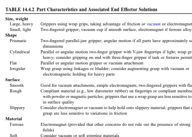
TABLE 14.4.2 Part Characteristics and Associated End Effector Solutions
Size, weight
Large, heavy Grippers using wrap grips, taking advantage of friction or vacuum or electromagnetic holding Small, light Two-fingered gripper; vacuum cup if smooth surface, electromagnet if ferrous alloy
Shape
Prismatic Two-fingered parallel-jaw gripper; angular motion if all parts have approximately same dimensions
Cylindrical Parallel or angular motion two-finger gripper with V-jaw fingertips if light; wrap gripper if heavy; consider gripping on end with three-finger gripper if task or fixtures permit Flat Parallel or angular motion gripper or vacuum attachment
Irregular Wrap grasp using linkages or bladder; consider augmenting grasp with vacuum or electromagnetic holding for heavy parts
Surface
Smooth Good for vacuum attachments, simple electromagnets, two-fingered grippers with flat fingertips Rough Compliant material (e.g., low durometer rubber) on fingertips or compliant membrane filled
with powder or magnetic particles; grippers that use a wrap grasp are less sensitive to variations in surface quality
Slippery Consider electromagnet or vacuum to help hold onto slippery material; grippers that use a wrap grasp are less sensitive to variations in friction
Material
Ferrous Electromagnet (provided that other concerns do not rule out the presence of strong magnetic fields)
Soft Consider vacuum or soft gripping materials
14-32 Section 14
Summary
In summary, we observe that end effector design and selection are inextricably coupled with the design of parts, robots, fixtures, and tooling. While this interdependence complicates end effector design, it also provides opportunities because difficult problems involving geometry, sensing, or task-related forces can be tackled on all of these fronts.
14.5 Sensors and Actuators
Kok-Meng Lee
Sensors and actuators play an important role in robotic manipulation and its applications. They must operate precisely and function reliably as they directly influence the performance of the robot operation. A transducer, a sensor or actuator, like most devices, is described by a number of characteristics and distinctive features. In this section, we describe in detail the different sensing and actuation methods for robotic applications, the operating principle describing the energy conversion, and various significant designs that incorporate these methods. This section is divided into four subsections, namely, tactile and proximity sensors, force sensors, vision, and actuators.
By definition, tactile sensing is the continuously variable sensing of forces and force gradients over an area. This task is usually performed by an m × n array of industrial sensors called forcels. By considering the outputs from all of the individual forcels, it is possible to construct a tactile image of the targeted object. This ability is a form of sensory feedback which is important in development of robots. These robots will incorporate tactile sensing pads in their end effectors. By using the tactile image of the grasped object, it will be possible to determine such factors as the presence, size, shape, texture, and thermal conductivity of the grasped object. The location and orientation of the object as well as reaction forces and moments could also be detected. Finally, the tactile image could be used to detect the onset of part slipping. Much of the tactile sensor data processing is parallel with that of the vision sensing. Recognition of contacting objects by extracting and classifying features in the tactile image has been a primary goal. Thus, the description of tactile sensor in the following subsection will be focused on transduction methods and their relative advantages and disadvantages.
Proximity sensing, on the other hand, is the detection of approach to a workplace or obstacle prior to touching. Proximity sensing is required for really competent general-purpose robots. Even in a highly structured environment where object location is presumably known, accidental collision may occur, and foreign object could intrude. Avoidance of damaging collision is imperative. However, even if the environment is structured as planned, it is often necessary to slow a working manipulator from a high slew rate to a slow approach just prior to touch. Since workpiece position accuracy always has some tolerance, proximity sensing is still useful.
Many robotic processes require sensors to transduce contact force information for use in loop closure and data gathering functions. Contact sensors, wrist force/torque sensors, and force probes are used in many applications such as grasping, assembly, and part inspection. Unlike tactile sensing which measures pressure over a relatively large area, force sensing measures action applied to a spot. Tactile sensing concerns extracting features of the object being touched, whereas quantitative measurement is of par-ticular interest in force sensing. However, many transduction methods for tactile sensing are appropriate for force sensing.
In the last three decades, computer vision has been extensively studied in many application areas which include character recognition, medical diagnosis, target detection, and remote sensing. The capabilities of commercial vision systems for robotic applications, however, are still limited. One reason for this slow progress is that robotic tasks often require sophisticated vision interpretation, yet demand low cost and high speed, accuracy, reliability, and flexibility. Factors limiting the commercially available computer vision techniques and methods to facilitate vision applications in robotics are highlights of the subsection on vision.
Tactile and Proximity Sensors
14-34 Section 14
loads ranging from 0 to 1000 g, having a 1-g sensitivity, a dynamic range of 1000:1, and a bandwidth of approximately 100 Hz. Furthermore, forcers should be spaced no more than 2 mm apart and on at least a 10 × 10 grid. A wide range of transduction techniques have been used in the designs of the present