An Assessment of Potential of Mean Force Calculations with Implicit Solvent Models
Collin M. Stultz*
HarVard-MIT DiVision of Health Sciences and Technology, and Department of Electrical Engineering and Computer Science, Massachussetts Institute of Technology, The Stata Center, 32-310, 32 Vassar Street, Cambridge, Massachussetts 02139
ReceiVed: June 30, 2004; In Final Form: August 16, 2004
An adequate representation of aqueous solvent is a fundamental problem in the field of macromolecular simulations. To assess the ability of different solvent models to reproduce experimental data, we performed a series of molecular dynamics simulations on a small peptide, each utilizing a different model of solvent. The generalized Born (GB) model, the analytical continuum electrostatics (ACE) potential, the effective energy function-1 (EEF1), the solvent accessible surface area (SASA) model, and the standard TIP3P model of explicit solvent were evaluated in this study. For each solvent model, the potential of mean force (pmf) for folding a 12-residue peptide from the fully extended state to a compact state, where the two ends of the pep-tide are in close proximity, was computed. These data were compared to experimental results on the peppep-tide’s end-to-end distance distribution obtained with fluorescent resonance energy transfer (FRET) experiments. For each solvent model, the FRET efficiency was computed from the corresponding pmf and compared to the experimental result. The value obtained from the simulation with explicit solvent was in excellent agreement with experiment. By contrast, all simulations that employed an implicit solvent model yielded values for the FRET efficiency that significantly deviated from the experimental value. An analysis of the energetic contributions to the pmf suggests potential etiologies for this marked discrepancy from experiment.
1. Introduction
Solvent plays a critical role in defining the conformational landscape of proteins and nucleic acids. Consequently an accurate representation of water is an essential component of meaningful biomolecular simulations.1,2Since dynamical
simu-lations with explicit solvent may be computationally intensive, considerable effort has been directed at deriving energy functions that adequately reproduce the same information in a fraction of the CPU time. A number of such implicit solvent models have been developed and key insights into the folding mechanism of several proteins have been obtained with these methods.3,4
While it is clear that many of these approaches can qualitatively reproduce important features of macromolecular thermodynam-ics and dynamthermodynam-ics,3few studies have attempted to delineate the
limitations of such models with respect to their ability to quan-titatively reproduce experimental data. In light of this, we as-sessed the ability of different implicit solvent models to ade-quately reproduce a known, experimentally determined, quantity. The implicit solvent models examined in the present study represent a range of methods that have gained acceptance in the field of macromolecular simulations. One model, the generalized Born (GB) approach, is an application of the Born equation for ionic solvation to polyatomic molecules.5-7Using
a linearized form of the GB equation introduced by Still et al.,6
Dominy and Brooks parametrized the GB model for proteins and nucleic acids.8In a subsequent work, the force field was
used to calculate the potential of mean force (pmf) for the folding of a 20-residueβ-sheet protein and the resulting data were in qualitative agreement with the pmf computed with the TIP3P model of explicit solvent.9Although the locations of the
global energy minima and saddle points were in approximate
agreement between the two models, important quantitative differences were noted; e.g., the stability of the native state was overestimated in the GB model.9These results demonstrate the
utility of the method for calculating free energy profiles; however, the lack of quantitative agreement between the two approaches suggests that quantitative data arising from such simulations should be interpreted with care.
In a related approach, Schaefer and Karplus combined an integral equation method for the calculation of self-energies and the generalized Born equation to yield the analytical continuum electrostatics (ACE) potential.10 In a recent application, the
method was shown to yield stable trajectories on the order of 1 nanosecond for two homologousR/βproteins.11When combined
with an adaptive umbrella sampling approach and a nonpolar solvation term, simulations with the ACE potential yielded helix and sheet propensities, for a predominantly R-helical and a predominantlyβ-sheet protein, that were in good agreement with experiment.12 Moreover, the calculated3J
NHRspin-spin
cou-pling constants were in good agreement with values obtained from NMR studies.12The method has broad appeal, but remains
untested with regard to the precise calculation of free energy differences.
In a different approach, a Gaussian solvent-exclusion model was developed for the calculation of solvation free energies and incorporated into the CHARMM force field.13 This effective
energy function (EEF1) assumes that the solvation energy of a group is equal to the solvation free energy of that group in a small model compound minus the amount of solvation the group loses by being in contact with other atoms within the protein.13
In its initial implementation, thermodynamic parameters for the model were adapted from previously published values on model compounds14,15and long-range electrostatic effects were
mod-eled with a distance-dependent dielectric constant and neutral-* E-mail: [email protected].
16525 J. Phys. Chem. B 2004, 108, 16525-16532
ized “charged” side chains.13The potential has been used to
calculate folding trajectories of a smallR/βprotein, CI2, and to accurately discriminate between native and misfolded states in established sets of native-misfolded pairs.16,17 Given its
computational efficiency, the method holds considerable prom-ise. However, since charged moieties are neutralized, it is unclear whether the approach can adequately model features that involve interactions between charged side chains. Although it appears to work quite well for deciphering overall “coarse-grained” properties, it may not be appropriate for the calculation of free energy differences between states with different but similar conformations.
In a later work, Caflisch and co-workers developed an analogous implicit solvent potential that neutralizes charged side chains and employs a distance-dependent dielectric to model the dielectric screening effect of solvent. An additional term based on the popular solvent accessible surface area (SASA) approximation of Eisenberg and McLachlan was used to model the hydrophobic effect.18,19Since a number of methods exist
for the rapid estimation of an atom’s solvent accessible surface,20
algorithms that employ such approximations may, in principle, be extremely efficient. Such approaches have been applied to several small systems and fruitful results have been ob-tained.18,21,22 Nevertheless, few studies have systematically
examined the limitations of this approach. In a recent study, Shimizu et al., investigated the ability of an implicit solvent model, based on a solvent accessible surface area approximation, to reproduce an explicit water simulated three-body potential of mean force and found that the implicit solvent pmf did not reproduce the explicit solvent result.21These data highlight the
fact that such models may not be appropriate for the calculation of some thermodynamic parameters.
Explicit solvent models have been used extensively to study the dynamics and thermodynamics of different biomolecular systems with considerable success. While it has been shown that such models may not accurately reproduce all the physical characteristics of bulk solvent,23a number of studies utilizing
models of explicit solvent have obtained results that agree with experiment.24 Recently we used the TIP3P model of explicit
solvent to calculate the pmf for the folding of a small 12-residue peptide that forms the flexible N-terminal autoregulatory region of tyrosine hydroxylase.25In a complementary set of
experi-ments, the fluorescent resonance energy transfer (FRET) ef-ficiency was measured for the peptide in solution.25In that work,
we demonstrated how FRET efficiencies could be calculated from the pmf and showed that the calculated FRET efficiency was in excellent agreement with the experimentally determined value. In the present study we extend these results by calculating free energy profiles with the implicit solvent models described above and compare the calculated FRET efficiencies to the experimental result. These data highlight the limitations of implicit solvent models with regard to the calculation of this macroscopic quantity.
2. Methods
FRET Measurements. The peptide of interest corresponds to amino acids 24-33 of rat tyrosine hydroxylase:26
KQAE-AVTSPR. FRET measures the energy transferred between two fluorescent pharmacophoressa donor and an acceptorsthat have been added to the peptide/protein of interest.27In this study, a
dansyl group was used as the acceptor group and the indole side chain of tryptophan was used as the donor group. The FRET efficiency, E, is defined as the number of energy transfer events divided by the number of photons absorbed by the donor27and
was calculated from measurements of the emission spectrum of the peptide.25Peptide synthesis and purification was
formed by Genemed Synthesis and measurements were per-formed as described in our prior work.25
Molecular Dynamics Simulations with Explicit Solvent. An extended-carbon polar-hydrogen model of the peptide KQAEAVTSPR peptide was constructed using the CHARMM program.28The FRET calculations utilized peptides that were
labeled with a dansyl group on the N-terminus and a tryptophan residue on the C-terminus. Since the CHARMM parameter set does not contain parameters for a dansyl group, we placed a tryptophan residue on both the N and C-termini of the peptide. This substitution was expected to yield results that would be comparable to the data obtained in the FRET measurements because both dansyl and tryptophan are composed of large aromatic moieties. Moreover calculations employing a tryp-tophan at both ends of the molecule showed excellent agreement with experiment.25Initial coordinates for the peptide,
KQAE-AVTSPR, were built using the IC facility of CHARMM.28
Details of the molecular simulations with explicit solvent were presented in our prior work,25 hence, we briefly outline the
approach here.
The calculations began with the fully extended conformation of the peptide. The peptide model was minimized for 100 steps of steepest descent minimization using a distance-dependent dielectric to minimize any unfavorable atomic overlaps within the structure. The extended structure was then overlaid with a set of 1000 equilibrated TIP3P water molecules,28and waters
that overlapped with the structure were removed. The remaining water molecules were equilibrated in the field of the fixed peptide structure with 100 steps of steepest descent minimization followed by 5 ps of standard molecular dynamics at 300 K. Repeated cycles of solvent overlay followed by minimization yielded a total of 1649 water molecules that were added to the structure. Molecular dynamics simulations employed a non-bonded cutoff of 13 Å. van der Waals interactions were switched to 0 between 10 and 12 Å and electrostatic interactions were shifted to 0 at a distance of 12 Å. Water molecules were restrained to lie within a sphere of radius 30 Å surrounding the peptide of interest using a stochastic boundary potential.29All
simulations were performed at 300 K using a Nose-Hoover thermostat30,31as implemented in CHARMM.28
For these calculations the end-to-end distance was defined as the distance between the CR carbons of each tryptophan residue located at each end, i.e., the reaction coordinate,ζ. At each simulation window,ζwas restrained to a specified distance using a harmonic biasing potential with a force constant of 25 kcal/mol/Å2. The first window began with the fully extended
state which corresponds toζ)36.4 Å. Each subsequent window began with an end-to-end distance that was 0.5 Å less than the prior value; e.g., windows were centered at 36.4, 35.9, 35.4, 34.9, 34.5...6.9 Å. A total of 60 windows were performed. Each window consisted of 20 ps of equilibration followed by 20 ps of production dynamics. The value of the reaction coordinate during the simulations was saved every 0.01 ps; yielding 2000 data points per window. The pmf at each window i, Gi(ζ), was calculated from the resulting frequency distribution, pi, and the biasing potential, Vi(ζ), using the equation Gi(ζ)) -kT ln pi -(ζ)-Vi(ζ)+Ci, where Ciis a function of the temperature, T, and the biasing potential, Vi(ζ).25,32 Representative average structures for each window were generated using the COOR facility in CHARMM.28Average structures were energy
The pmfs arising from the different windows were linked to form one continuous pmf over the entire range of end-to-end distances using an automated procedure as implemented in the program SPLICE.32Briefly, the potentials of mean forces from
two sequential windows were linked by first comparing the overlapping regions to find a common point where the potentials had similar slopes. The second potential was then adjusted to agree with the first at this common point. The final potential of mean force was smoothed using the moving average window method with a window span of 3. Smoothing did not affect the positions of saddle points or energy minima for either potential of mean force.
For each of the solvent models analyzed in this work, the umbrella sampling windows, restraining potentials, and proce-dure for splicing the various windows together to form one con-tinuous potential of mean force were identical to that described above. Below we discuss computational issues that are specific to each model. In particular, the nonbond cutoff for each implicit solvent model was chosen based on previously published work. The goal was to maximize the likelihood that a given solvent model would reproduce the explicit solvent results.
Molecular Dynamics Simulations with GB. GB simulations utilized the method implemented by Dominy and Brooks within the CHARMM program.8In their previous work, the GB model
was used to calculate the folding free energy landscape for a smallβ-sheet protein and qualitative agreement with explicit solvent simulations was obtained.9 In that study, all pairwise
interactions were included in each of the GB simulations and no cutoffs were used. Therefore, we follow the same approach and conduct all of our GB calculations without any truncation of the nonbond interactions.
Molecular Dynamics Simulations with ACE. The ACE potential as implemented in the CHARMM program was utilized in this work.10Prior work suggests that the ACE potential with
standard nonbond cutoffs yields agreement with experimental data on helix and sheet propensities and measured3J
NHRspin
-spin coupling constants.12We follow a similar approach and
employ electrostatic and van der Waals cutoffs tidentical to those used in the explicit solvent simulations. The implementation of ACE employed in this work also utilized a nonpolar solvation term as previously described.12
Molecular Dynamics Simulations with EEF1. The EEF1 potential, as previously described, was used in this work.13Since
the nonbond cutoffs for the EEF1 potential are part of the model, they are predetermined as specified in the original implementa-tion; i.e., van der Waals interactions were switched to 0 between 7 and 9 Å and electrostatic interactions were shifted to 0 at a distance of 9 Å. Charged side chains were neutralized as previously described.13
Molecular Dynamics Simulations with SASA. The SASA potential as implemented in CHARMM29 was used in this work.18Since SASA is based, in part, on the EEF1 potential,
its nonbond cutoffs are identical to those used in the EEF1 potential.18
Calculating the FRET Efficiency from the PMF. The FRET efficiency was calculated from the potential of mean force as described in our preceding work.25Here we briefly review
the procedure employed for these calculations.
If the donor and acceptor are separated by a fixed distance,
ζ, then the FRET efficiency can be written as27
where R0denotes the Fo¨rster critical distance; i.e., the distance
at which E is equal to 0.5. For the dansyl/tryptophan pair, R0
equals 23.6 Å.27In the case of flexible peptides, the
interpreta-tion of the FRET efficiency is not straightforward. Since most peptides can adopt a number of distinct conformational states in solution, the observed emission spectra correspond to an average of the different spectra from all of the peptide’s accessible conformational states. Thus for peptides, the statistical mechanical expression for the FRET efficiency becomes
It follows that the FRET efficiency can be calculated from the pmf using the relationship
where m and M denote the minimum and maximum values for the end-to-end distance for the peptide of interest and G(ζ) denotes the pmf as a function of the end-to-end distance.25
FDPB Calculations. To determine how results from the various implicit solvent models compare to results obtained with a standard continuum electrostatic model, we calculated the electrostatic solvation energy of representative structures using the linear Possion-Boltzmann equation as implemented in the program UHBD.33The structures chosen for the UHBD
calcula-tions are described in the text. The solvation energy of each structure is the energy associated with transferring the peptide from low dielectric medium where)1 to a high dielectric medium where)80. For each structure, the solvation energy was computed using a focused grid spacing of 0.21 Å in a manner similar to that previously described.10
3. Results and Discussion
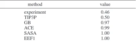
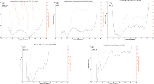
[image:3.612.320.558.58.132.2]Comparison of the Implicit and Explicit Solvent pmfs. The experimentally measured FRET efficiency is in excellent agreement with the result obtained using a TIP3P model of solvent; i.e., the explicit solvent pmf (Table 1). The fact that the calculated FRET efficiency agrees with the experimentally determined value argues that the explicit solvent simulations adequately describe the experimental conditions. By contrast, the calculated FRET efficiencies from the implicit solvent pmfs significantly differ from the experimentally determined value and, not surprisingly, the implicit solvent pmfs themselves differ from the explicit solvent profile (Figure 1A-E, dark lines). Of the four implicit solvent models, the GB and ACE potentials are most similar to the explicit solvent pmf. The TIP3P, GB, and ACE pmfs all contain states with end-to-end distances between 5 and 25 Å that have energies within 5 kcal/mol of the lowest energy state (Figure 1A, B, and C). However, the free energy profiles generated with the EEF1 and SASA models TABLE 1: Measured and Calculated FRET Efficiencies
method value
experiment 0.46
TIP3P 0.50
GB 0.97
ACE 0.99
SASA 1.00
EEF1 1.00
E(ζ)) R0 6
R06+ζ6
E)
〈
R0 6R06+ζ6
〉
)〈E(ζ)〉
E≈
∫
m ME(ζ)e-G(ζ)/kTdζ
∫
m Mare significantly differentsboth have prominent minima near 6 Å and a rapidly increasing energy fromζ)10 to 25 Å.
The TIP3P pmf contains three prominent local energy minima located at approximately 9, 11, and 24 Å, where the minimum near 24 Å corresponds to the lowest energy state (Figure 1A). The implicit solvent pmfs, however, have low energy states with end-to-end distances that are significantly smaller than 24 Å (Figure 1B-E). The lowest energy states for the GB and ACE potentials, methods based on the generalized Born equation, have global energy minima with end-to-end distances near 10 Å (Figure 1B and C). Likewise, the EEF1 and SASA potentials, methods that neutralize charged side chains, have more compact lowest energy states with end-to-end distances in the vicinity of 6 Å (Figure 1D and E).
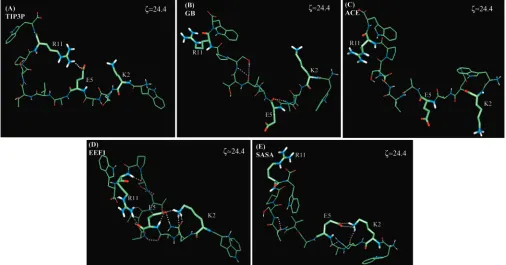
The peptide of interest contains five charged groups: an N-terminus, Lys 2, Glu 5, Arg 11, and a C-terminus. Since these charged moieties are expected to be well solvated in the peptide, it is likely that the particular solvent model used will have a significant impact on the local conformation of these groups. To gain insight into the physical basis behind the differences in the form of the pmfs, we examined representative structures from each free energy profile to determine how the structure of these charged groups, and the peptide as a whole, are affected by the particular model of solvent. The lowest energy state from the explicit solvent pmf has a well-defined minimum atζ )
24.4 Å (Figure 1A), and more than 90% of the structures arising from the simulation centered at 24.4 Å contain a salt bridge between Glu 5 and Arg 11 (Figure 2A).25However, the lowest
energy states arising from the GB and ACE potentials cor-respond to conformations that do not contain a salt bridge between any charged groups (Figure 2B and C). The only hydrogen bond involving a charged side chain is formed in the GB model and involves the side chain of Arg 11 and the backbone carbonyl of Lys 2. All other charged groups are solvent exposed and do not interact with other moieties within the peptide.
Although simulations with the EEF1 and SASA potentials result in the formation of a number of hydrogen bonds between polar moieties, including a salt bridge between Glu 5 and Lys 2, the salt bridge that occurs in the explicit solvent simulations never forms (Figure 3D and E). The lowest energy states from the EEF1 and SASA potentials are more compact, and repre-sentative structures from simulations centered at these end-to-end distances (ζ)6 Å) have significantly more hydrogen bonds between the various polar groups (Figure 2D and E). Moreover, virtually all charged groups hydrogen bond to other polar moieties in the peptide. As charged groups are neutralized in these models, the Coulombic contribution to the potential energy from two charged groups is similar to that which arises from hydrogen bonds between uncharged, polar moieties. It follows that charged groups in this model form hydrogen bonds in a manner similar to that of uncharged polar moieties.
This analysis suggests that models based on the generalized Born approach (i.e., ACE and GB), have low energy structures where charged residues prefer solvent exposed conformations, and methods that employ neutralized side chains (i.e., EEF1 and SASA) have compact low energy structures where charged side chains are involved in multiple hydrogen bonds with polar moieties.
Explaining the Difference between the Calculated FRET Efficiencies. If a fluorescent donor and acceptor are separated by a fixed end-to-end distance,ζ, the FRET efficiency is given by
where R0denotes the Fo¨rster critical distance (23.6 Å for a
dansyl-tryptophan pair).27If the molecule of interest has a fixed
[image:4.612.60.553.47.318.2]end-to-end distance of 24 Å the corresponding FRET efficiency is 0.47sa value close to the experimentally determined value of 0.46.
Figure 1. Potential of mean force (pmf) for the different solvent models analyzed in this work (solid dark line). Each plot is labeled with the
solvent model used for that simulation. The average potential energy as a function of the end-to-end distance is depicted as a dotted red line in each plot.
E(ζ)) R0 6
The dominant state of the explicit solvent pmf has an end distance near 24 Å and therefore the calculated end-to-end distance is close to the experimental value of 0.46. As the most favorable end-to-end distances in the implicit solvent pmfs are smaller, the FRET efficiencies from the implicit solvent models are significantly larger; i.e., energy transfer is much more efficient when the ends are in close proximity. Since the correct calculation of the FRET efficiency is likely dependent on the presence of a prominent minimum at approximately 24 Å, the failure of the implicit solvent models to mimic the experimental data can be explained, in part, by the fact that each implicit
solvent pmf lacks a well-defined minimum near 24 Å. Therefore, to understand why each implicit solvent model does not reproduce the experimentally determined FRET efficiency, we explore why the implicit solvent pmfs have global energy minima far from 24 Å.
[image:5.612.55.560.47.323.2]To determine the relative importance of the enthalpy and the configurational entropy in each pmf, we computed the average potential energy as a function of the end-to-end distance (Figure 1A-E, red dotted lines). We note that fluctuations in the potential energy of the TIP3P simulations are larger than fluctuations in the implicit solvent simulations. This is due to Figure 2. (Representative structures from the lowest free energy state in each solvent model.
[image:5.612.54.560.344.609.2]the fact that the explicit solvent calculations included over 1000 TIP3P molecules, and therefore the total energy of the system, is significantly larger than the energies arising from the implicit solvent models. Nevertheless, although the rms fluctuations are larger, these fluctuations represent a small fraction of the total energy of the system.
All implicit solvent pmfs have global energy minima within 5 Å of the state of lowest potential energy (Figure 1B-E). By contrast, the lowest energy state from the explicit solvent model is separated from the state of lowest potential energy by more than 15 Å (Figure 1A). These findings suggest that enthalpic contributions dominate the position of the global energy minimum in the implicit solvent pmfs, whereas the configuration entropy of the peptide plays an important role in stabilizing the lowest energy state in simulations with the TIP3P model of explicit solvent. An analysis of representative structures from the global energy minimum positions in the implicit solvent pmfs (Figure 2B-E) reveals that low energy states from the implicit solvent simulations have considerably more hydrogen bonds relative to the state corresponding toζ)24.4 Å (Figure 3B-E). As the enthalpy appears to be an essential determinant of the position of the lowest energy state, compact states containing multiple hydrogen bonds dictate the position of the lowest free energy state.
Comparison with FDPB Calculations. A number of implicit solvent models have been developed and parametrized based on data obtained from finite difference Poisson-Boltzmann (FDPB) methods.3Since Poissson-Boltzmann calculations have
been shown to agree with experimentally determined solvation energies of small compounds, ensuring that novel implicit solvent methods agree with FDPB calculations guarantees that the resulting potentials will yield accurate values for small groups such as amino acid side chains and peptide backbone analogues.34In its initial implementation, parameters for the GB
model were obtained, in part, by ensuring that calculations of the GB polarization energy yielded Born radii that were similar to radii obtained with FDPB calculations.8Likewise, previous
work has demonstrated that ACE solvation energies for small compounds were similar to that obtained with FDPB calcula-tions.10As such, both models, in principle, produce solvation
energies for small molecules that are comparable to what would be obtained with FDPB. Therefore, for these calculations, we focus on the GB and ACE potentials to determine if FDPB calculations would also yield results that were similar to the GB and ACE findings.
The GB and ACE simulations both suggest that structures containing a salt bridge between Glu 5 and Arg 11 are relatively unfavorablesa finding at odds with the explicit solvent result. To determine whether the relative PB energy of these structures would agree with the GB and ACE results, we compared the electrostatic energies of conformations arising from the explicit solvent simulations centered atζ)24.4 (e.g., Figure 3A) to corresponding structures obtained with the GB and ACE potentials (e.g., Figure 3B and C).
Ten structures were chosen from each of the TIP3P, GB, and ACE simulations centered atζ)24.4Å; one structure every 2 ps. For each of the TIP3P structures, all water molecules were deleted and the structures of the peptide were used for the solvation energy calculations. The collection of representative structures from the TIP3P simulation is denoted by{ζ)24.4}ER
where the superscript ER is used to emphasize the fact that Glu 5 and Arg 11 form a salt bridge in all 10 structures. Similarly, the collection of 10 structures from the GB and ACE simulations are denoted by{ζ)24.4}GBand{ζ)24.4}ACE, respectively.
None of the representative structures from the GB and ACE simulations contain hydrogen bonds to charged groups (e.g., Figure 3B and C). To determine how FDPB solvation energies compare to the GB and ACE results we computed the electrostatic energy of the representative structures in each data set using a FDPB algorithm as implemented in the program UHBD.33The FDPB solvation energy is defined as the average
FDPB energy of the 10 structures in{ζ)24.4}ER, similarly,
the GB and ACE solvation energies were defined as averages over their corresponding structure sets. The results are expressed as the difference between the electrostatic energy of the set containing the salt bridge,{ζ)24.4}ER, and the electrostatic
energy of sets containing structures with exposed side chains; i.e.,{ζ)24.4}GBand{ζ)24.4}ACE.
Both the GB and ACE results suggest that conformations with exposed side chains have more favorable electrostatic energies than structures containing the salt-bridge of interest (Table 2). Moreover, the FDPB calculations yield electrostatic free energy differences that are similar to those obtained with the GB and ACE potentialsswith the GB result begin closest to the FDPB results (Table 2). As such, FDPB, GB, and ACE all suggest that conformations containing a Glu 5 to Arg 11 salt-bridge are less stable than corresponding structures with no charge -charge interactions.
Structures arising from the TIP3P simulations centered atζ
)24.4 contain a salt bridge, whereas structures arising from the GB and ACE simulations do not. To assess how the formation of an individual salt bridge influences our results, we computed the electrostatic binding energy associated with the formation of the salt bridge between Glu 5 and Arg 11. For these calculations, the orientations of the Glu 5 and Arg 11 residues were obtained from the{ζ)24.4}ER data set; i.e., a
collection of 10 coordinate files, each one containing only the coordinates for Glu and Arg, was constructed from {ζ )
24.4}ER. Each coordinate file in this collection contains the
conformation of a salt bridge involving a Glu and an Arg residue. For each salt-bridge configuration, the electrostatic binding energy was computed using the thermodynamic path shown in Figure 4 and the results are listed in Table 3. Each entry represents the average over the 10 different salt-bridge configurations taken from the{ζ)24.4}ERstructure set.
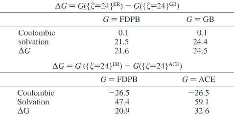
[image:6.612.318.557.70.192.2]Although the GB and ACE solvation energies are similar to the FDPB results, only the FDPB calculations predict that formation of the Glu-Arg salt bridge is favorable. Nonetheless, the calculated binding energy is smallsonly-0.7 kcal/mol, a value similar to kT at room temperaturessuggesting that the salt bridge is only marginally stable (Table 3). However, the GB electrostatic binding energy suggests that the formation of the Glu-Arg salt bridge is unfavorable. The discrepancy between the two results is explained by the difference in the solvation energies of the Glu residue and the Glu-Arg pair TABLE 2: Electrostatic Free Energy Difference,∆G, of
Conformations from Various Solvent Models (in kcal/mol)
∆G)G({ζ)24}ER)-G({ζ)24}GB)
G)FDPB G)GB
Coulombic 0.1 0.1
solvation 21.5 24.4
∆G 21.6 24.5
∆G)G ({ζ)24}ER)-G({ζ)24}ACE)
G)FDPB G)ACE
Coulombic -26.5 -26.5
Solvation 47.4 59.1
(Table 3). Similar results are noted for the ACE potential, however, the ACE electrostatic binding energy deviates more from the FDPB result (Table 3). Again, the etiology of this difference is explained, almost exclusively, by the less favorable solvation energy of the Glu-Arg pair. Nevertheless, of the two implicit solvent models, the GB result is closest to the FDPB calculation.
4. Conclusions
A number of studies have demonstrated the utility of implicit solvent models for obtaining structural information on biomol-ecules. The main advantage of such methods is that they simulate trajectories in a fraction of the time that would be required for comparable simulations with explicit solvent.1,3
Such methods have been used to calculate folding trajectories of small proteins,4,9,16to discriminate between correctly folded
and misfolded states,17and to understand the solution dynamics
of a variety of peptides and proteins.3,12,21 As such, these
methods have an important role in the study of proteins and nucleic acids.
The objective of this work was to evaluate how well several of these models perform with regard to the calculation of a specific macroscopic observablesthe FRET efficiency. The calculated FRET efficiency from the explicit solvent pmf is in excellent agreement with the experimental value, while the calculated values from each implicit solvent pmf markedly differs from the experimental result. Moreover, all of the solvent models investigated here, including the TIP3P model, have enthalpic minima with end-to-end distances below 15 Å. The main difference between the implicit solvent model and the TIP3P model is that the global free energy minimum for each implicit solvent model lies near the state of lowest enthalpy, whereas the explicit solvent pmf has a global free energy minimum that is more than 10 Å from the state of lowest enthalpy. This suggests that the enthalpy dominates the position of the global free energy minimum in the implicit solvent models, but the entropy plays a significant role in defining the position of the explicit solvent global free energy minimum.
The pmf is the free energy as a function of the peptide’s end distance. Extended states, with relatively large end-to-end distances, have larger configurational entropies. As such, there is an implicit dependence of the entropy on the length of the polymer. By contrast, the enthalpy of the peptide is determined by the formation of close, energetically favorable contacts (e.g., hydrogen bonds, salt bridges). Therefore, the enthalpy favors the formation of more compact states. In particular, if all the interatomic interactions were turned off, the simulations would favor extended states as the entropic term would then dominate. It follows that the extent to which more compact states are favored is determined, in part, by the relative importance of the enthalpic contribution. As the implicit solvent models have global free energy minima with smaller end-to-end distances, these data suggest that the enthalpic contribution dominates the free energy profile for these models, while in the explicit solvent model, the configurational entropy of the peptide plays a more significant role. Representative structures from the lowest energy state in each pmf are consistent with these data in that the lowest energy states from the implicit solvent pmfs contain a significant number of hydrogen bonds and have a lower potential energy than corresponding structures from the explicit solvent simulations.
The explicit solvent pmf contains a well-defined minimum at approximately 24 Åsan end-to-end distance that corresponds to a FRET efficiency near the experimental value. The implicit solvent models, however, contain global energy minima at end-to-end distances that are significantly shorter, and this explains, in part, the significant deviation from the experimental value. The lowest energy state from the explicit solvent pmf contains a salt-bridge between a Glu and an Arg residue. By contrast, representative structures from each implicit solvent pmf that have an end-to-end distance of 24 Å do not contain the “correct” salt bridge relative to the structure obtained from the explicit solvent pmf. Moreover, representative structures arising from both the GB and ACE simulations atζ≈24 Å have charged side chains that are fully solvent exposedssuggesting that charged residues in the GB and ACE simulations prefer solvent exposed orientations.
Although the GB and ACE results differ from the explicit solvent data, these implicit solvent pmfs are more similar to the explicit solvent result than the EEF1 and SASA pmfs (Figure 1). The GB, ACE, and explicit solvent pmfs predict that a range of end-to-end distances have similar energies, whereas the EEF1 and SASA pmfs have a small number of low energy states with to-end distances below 10 Å. Structures with larger end-to-end distances have significantly larger energies (Figure 1). In earlier work, it was demonstrated that both the GB and ACE potentials yield solvation energies for small compounds that are similar to data obtained with FDPB.8,10FDPB
[image:7.612.55.296.52.139.2]calcula-tions on representative structures from the different solvent models yield electrostatic energy differences that are similar to data obtained from direct energy calculations using the GB and ACE potentials, with the GB results being closest to the FDPB energies. These calculations agree with prior data in that the GB and ACE calculations yield energies that are comparable to the FDPB result. However, it is interesting to note that the FDPB calculations incorrectly predict the peptide structure containing a salt bridge to be less favorable than the corre-sponding structure with solvent exposed side chains. As such, implicit solvent models that attempt to reproduce FDPB energies are doomed to incorrect predictions of the relative stability of different conformational states of this peptide. These results suggest that agreement with FDPB alone may be an inadequate Figure 4. Thermodynamic cycle used to calculate the electrostatic
binding energy,∆Ebind, for the formation of a salt bridge between a glutamate residue, E, and an arginine residue, R. The separated residues are transferred from solvent to vacuum and the associated free energies are-∆GsolEV and -∆GsolRV. The separated residues then form a salt bridge and the associated Coulombic interaction term is∆GCoul. The complex is then resolvated and the corresponding contribution is denoted by∆GsolERV. The overall electrostatic binding energy,∆Gbind, equals the sum of the contributions along each path.
TABLE 3: Electrostatic Binding Energy,∆Gbind, for the
Formation of a Salt Bridge (in kcal/mol)
contribution FDPB GB ACE
-∆GsolVE 78.6 81.9 74.5
-∆GsolVE 98.5 90.2 97.0
∆GCoul -73.8 -73.8 -73.8
∆GsolVER -104.0 -97.1 -93.6
[image:7.612.54.295.262.328.2]way to parametrize an implicit solvent model if such a model is to be used for the calculation of free energy differences.
As an aside, we note that in this study we were primarily concerned with conformations of the peptidesthe quantity that can be compared to an experimentally determined value. Con-sequently, we chose a reaction coordinate that could be easily related to the measured FRET efficiency. The contribution of the configurational entropy of the explicit solvent is not easily determined using this reaction coordinate, and therefore our analysis does not include an investigation into these affects. Nevertheless, we believe that important insights into the limitations of these different solvent models arise from this limited analysis.
Although the computational efficiency of implicit solvent models makes their application to a wide array of problems tempting, such an approach is likely not justified based on our results. In particular, estimates of detailed free energy differences between distinct conformational states may not be accurately obtained with such methods. Moreover, given that representative structures obtained from the implicit solvent pmfs significantly differ from corresponding structures taken from explicit solvent simulations, it is unclear whether these approaches, in their current implementation, are appropriate for the analysis of specific conformational changes in peptides. Given that the different models treat charged side chains in very different ways, the discrepancy between implicit solvent and explicit solvent results is likely to be most egregious for peptides and small proteins with several charged moieties.
It is important to remember that useful insights into the conformational dynamics of proteins and peptides have been obtained with a number of implicit solvent models, and their existence enables an analysis of protein trajectories on long time scales.3 As such they remain valuable tools in the arsenal of
molecular simulation algorithms. Our data, however, suggest that results obtained with such models need to be interpreted with care especially when they are used for the determination of detailed free energy differences.
Acknowledgment. I thank Martin Karplus, Elazer Edelman, and Andrew Levin for a critical reading of the manuscript. C.M.S. is a Burroughs Wellcome Fund Career Awardee in the Biomedical Sciences.
References and Notes
(1) Brooks, C. L.; Karplus, M.; Pettitt, B. M. Proteins: a Theoretical PerspectiVe of Dynamics, Structure, and Thermodynamics; Vol. 71 of
Advances in Chemical Physics series; John Wiley and Sons: New York, 1988.
(2) Levy, R. M.; Gallicchio, E. Annu. ReV. Phys. Chem. 1998, 49, 531. (3) Roux, B.; Simonson, T. Biophys. Chem. 1999, 78, 1.
(4) Brooks, C. L. Curr. Opin. Struct. Biol. 1998, 8, 222. (5) Born, M. Z. Phys. 1920, 1, 45.
(6) Still, W. C.; Tempczyk, A.; Hawley R. C.; Hendrickson, T. J. J. Am. Chem. Soc. 1990, 112, 6127.
(7) Qui, D.; Shenkin, P. S., Hollinger, F. P.; Still, W. C. J. Phys. Chem. A 1997, 101, 3005.
(8) Dominy, B. N.; Brooks, C. L. J. Phys. Chem. B 1999, 103, 3765. (9) Bursulaya, B. D.; Brooks, C. L. J. Phys. Chem. B 2000, 104, 12378.
(10) Schaefer, M.; Karplus, M. J. Phys. Chem. 1996, 100, 1578. (11) Calimet, N.; Schaefer, M.; Simonson, T. Proteins: Struct., Funct., Genet. 2001, 45, 144.
(12) Schaefer, M.; Bartels, C.; Karplus, M. J. Mol. Biol. 1998, 284, 835.
(13) Lazaridis, T.; Karplus, M. Proteins: Struct., Funct., Genet.s 1999, 35, 133.
(14) Makhatadze, G. I.; Privalov, P. L. J. Mol. Biol. 1993, 232, 639. (15) Privalov, P. L.; Makhatadze, G. I. J. Mol. Biol. 1993, 232, 660. (16) Lazaridis, T.; Karplus, M. Science 1997, 278, 1928.
(17) Lazaridis, T.; Karplus, M. J. Mol. Biol. 1998, 288, 477. (18) Ferrara, P.; Apostolakis, J.; Caflisch, A. Proteins: Struct., Funct., Genet. 2002, 46, 24.
(19) Eisenberg, D.; McLachlan, A. D. Nature 1986, 319, 199. (20) Hasel, W.; Hendrickson, T. F.; Still, W.C. Tetrahedron Comput. Methodol. 1988, 1, 103.
(21) Shimizu, S.; Chan, H. S. Proteins: Struct. Funct., Genet. 2002, 48, 15.
(22) Ferrara, P.; Caflisch, A. Proc. Natl. Acad. Sci. U. S. A. 2000, 97, 10780.
(23) Horn, H. W.; Swope, W. C.; Pitera, J. W.; Madura, J. W.; Dick, T. J.; Hura, G. L.; Head-Gordon, T. J. Chem. Phys. 2004, 120, 9665.
(24) Levy, R. M.; Gallicchio, E. Annu. ReV. Phys. Chem. 1988, 49, 531. (25) Stultz, C. M.; Levin, A. D.; Edelman, E. R. J. Biol. Chem. 2002, 277, 47653.
(26) Haycock, J. W.; Ahn, N. G.; Cobb, M. H.; Krebs, E. G. Proc. Natl. Acad. Sci. U. S. A. 1992, 89, 2365.
(27) Lakowicz, J. R. Principles of Fluorescence Spectroscopy; Plenum Press: New York, 1983.
(28) Brooks, B.; Bruccoleri, R.; Olafson, B.; States, D.; Swaminathan, S.; Karplus, M. J. Comput. Chem. 1983, 4, 187.
(29) Brooks, C.; Karplus, M. J. Mol. Biol. 1989, 208, 159. (30) Nose, S. J. Chem. Phys. 1984, 81, 511.
(31) Hoover, W. G. Phys. ReV. A., 1985, 31, 1695. (32) Stultz, C. M. J. Mol. Biol. 2002, 319, 997.
(33) Davis, M. E.; Madura, J. D.; Luty, B. A.; McCammon, J. A. Comput. Phys. Comm. 1991, 62, 187.