Comparing Equilibria for Game-Theoretic and Evolutionary
Bargaining Models
Shaheen Fatima
Department of ComputerScience University of Liverpool Liverpool L69 7ZF, U.K.
[email protected]
Michael Wooldridge
Department of ComputerScience University of Liverpool Liverpool L69 7ZF, U.K.
[email protected]
Nicholas R. Jennings
Department of Electronics andComputer Science University of Southampton Southampton SO17 1BJ, U.K.
[email protected]
ABSTRACT
Game-theoretic models of bargaining are typically based on the as-sumption that players haveperfect rationalityand that they always play an equilibrium strategy. In contrast, research in experimental economics shows that in bargaining between human subjects, par-ticipants do not always play the equilibrium strategy. Such agents are said to be boundedly rational. In playing a game against a boundedly rational opponent, a player’s most effective strategy is not the equilibrium strategy, but the one that is the best reply to the opponent’s actual strategy. Against this background, this pa-per studies the bargaining behavior of boundedly rational agents by using genetic algorithms. Since bargaining involves players with different utility functions, we have two subpopulations – one rep-resents the buyer, and the other reprep-resents the seller (i.e., the pop-ulation is asymmetric). We study the competitive co-evolution of strategies in the two subpopulations for an incomplete information setting, and compare the results with those prescribed by game the-ory. Our analysis leads to two main conclusions. Firstly, our study shows that although each agent in the game-theoretic model has a strategy that is dominant at every period at which it makes a move, the stable state of the evolutionary model does not always match the game-theoretic equilibrium outcome. Secondly, as the players mutually adapt to each other’s strategy, the stable outcome depends on the initial population.
1. INTRODUCTION
Existing game-theoretic models of bargaining [13, 14, 15] are predicated on the presumption that agents areperfectly rational, and that this rationality iscommon knowledge. The participants in these models compute the equilibrium strategy from a theoret-ical analysis of the game and always play that strategy. In con-trast, research in experimental economics [12] suggests that the per-fect rationality assumption does not apply in human settings. This research shows that human participants learn how to play games through trial and error, and do not compute the equilibrium from a theoretical analysis of the game. Rather, they experiment with
Permission to make digital or hard copies of all or part of this work for personal or classroom use is granted without fee provided that copies are not made or distributed for profit or commercial advantage and that copies bear this notice and the full citation on thefirst page. To copy otherwise, to republish, to post on servers or to redistribute to lists, requires prior specific permission and/or a fee.
AAMAS-03 Workshop on Agent-Mediated Electronic Commerce V (AMEC-V)2003 Melbourne, Australia.
strategies, observe their payoffs, try other strategies andfind their way to a strategy that works well. Such players are said to be
boundedly rational. This result means game theory cannot always be used as a guide to behavior. An agent’s optimal actions may be quite different depending upon whether it is playing against a perfectly rational agent or a boundedly rational person.
This divergence led to the use of evolutionary methods for study-ing the bargainstudy-ing behavior of boundedly rational agents [18, 9, 4, 17, 1, 3]. Although for certain games the game-theoretic and evolutionary equilibria coincide [17, 16], in general, it has been shown that the game-theoretic outcome may not always be valid when playing against boundedly rational agents [2]. For instance, [18] and [4] show this in their evolutionary model for the Nash de-mand game, as do Binmore et al [1] in their evolutionary analysis of Rubinstein’s alternating offers game of complete information [13] that has a sub-game perfect equilibrium. Generally speaking, how-ever, this existing work comparing game-theoretic and evolutionary outcomes is based on two main assumptions. Firstly, agents have complete information about the bargaining parameters. Secondly, agents are drawn from a single population, in which all individu-als have the same utility function. However, we believe both of these assumptions are unlikely to be true in most practical applica-tions. To rectify this shortcoming, our objective in this paper is to assess to what extent the evolutionary computation of agent strate-gies matches the game-theoretic results for more realistic scenarios. Thus, we focus not only on an incomplete information setting, but also treat the population as asymmetric.
Specifically, the bargaining behavior of boundedly rational play-ers is studied using genetic algorithms (GAs) in which the popula-tion is composed of two separate subpopulapopula-tions – one representing the buyer and the other representing the seller. We use such asym-metric populations because buyers and sellers have fundamentally different aims and objectives (here represented by different utility functions). Moreover, the buyer and the seller each have time con-straints in the form of a deadline and a bargaining cost. In this model, which has been analysed game-theoretically in [7], each agent has a unique strategy that is dominant at every time period at which it makes a move.
0.4 0.6 0.8 1 psi=1
psi=10 psi=50
psi=0.1
psi=0.02
b b
b
t / T Price
0.2 RP
[image:2.612.331.539.8.123.2]IP
Figure 1: Negotiation decision functions for the buyer.
population on the stable state of the evolutionary model. The re-sults we obtain can then be used to select between the approaches for agent mediated electronic commerce applications, since this de-cision making involves not only a comparison of the outcomes they generate but also the feasibility of their implementation.
The remainder of the paper is structured as follows. Section 2 gives an overview of our negotiation model. The equilibrium out-comes for this model are presented in Section 3. Section 4 explains the evolutionary system. The results of our experiments are de-scribed in Section 5. Section 6 discusses related work and Section 7 gives some conclusions and states our future work.
2. THE NEGOTIATION MODEL
We assume that a buyer and a sellerbargain over the price
of a good/service. Each agent has an initial price () at which
it starts negotiation and a reservation price ( ) beyond which it does not concede. Let denote the range of values for
price that are acceptable to agent, where ;denotes
agent’s opponent. A price that is acceptable to both and,
i.e., the zone of agreement, is the interval
. The
difference between
and
is called theprice-surplus. denotes agent’s deadline. Let
denote the price offered by
toat time. We use an alternating offers protocol for our study.
Negotiation starts when thefirst offer is made. When an agent, say, receives an offer at time, i.e.,
, it rates the offer using
its utility function . If
is greater than the utility
of the counter-offer agentis ready to send at time
, i.e.,
¼
with
, then agentaccepts. Otherwise a counter-offer is
made. This process of making offers and counter-offers continues until either an agreement is reached, or a deadline is reached.
Since both agents have a deadline, we assume that they use a time dependent tactic (i.e., linear, Boulware, or Conceder [5]) for generating offers. These tactics vary the price depending on the remaining negotiation time. In these functions, the predominant factor used to decide which value to offer next is the time. The
initial offer is a point in the interval . Agents define
a constant , that, when multiplied by the size of the interval,
determines the price to be offered in thefirst proposal by. The
offer made byat time( ) is defined in terms of the
negotiation decision function (NDF), , as follows:
for
for.
A wide range of functions can be defined by varying the way in which is computed. However, functions must ensure that
, and . That is, the offer
Ts Tb
Ss
Sb
Ts Tb
Ss
Sb
RP
RP IP IP
O2 O
1
Price (a) Price (b)
Time
s
b b s
Figure 2: Illustration of agreement and negotiation conflict.
will always be between the value range, at the beginning it will give the initial constant, and when the deadline is reached it will offer the reservation value. The function is defined as follows:
½
An infinite number of functions can be defined for different val-ues of. However, the following two extreme sets show clearly
different patterns of behavior [11] (see Figure 1).
1. Boulware(B). For this function , and the initial offer
is maintained till time is almost exhausted, when the agent concedes up to its reservation value.
2. Conceder(C). For this function , and the agent goes
to its reservation value very quickly1. When
, price is
increased linearly (L).
The value of a counter-offer depends on the initial price (IP) at which the agent starts negotiation, thefinal price (FP), beyond which it does not concede,, and . A tuple, , of these four variables,
i.e., , forms agent’sstrategy. The
ne-gotiation outcome is an element of
, where ()
denotes thepriceandtimeof agreement and
denotes the conflict
outcome.
As an illustration, when
and
, the outcomethat results is shown in
Fig-ure 2. In thisfigure, and in all subsequent ones, the thick lines de-note ’s strategy and the dashed lines dede-note’s strategy. As shown
in thefigure, agreement (
) is reached at a price
-and at a time close to
. But when the NDF in both strategies is replaced with C, agreement (
) is reached at
the same price but near the beginning of negotiation. Figure 2(b) illustrates a negotiation conflict; where the strategies for and
are
, and
. As agents have different deadlines and both agents use thefunction, the strategies do not converge and result in a con-flict. In general, an agent can avoid conflict by using a strategy that offers a mutually acceptable price (i.e., within) by a mutually
acceptable time (the earlier deadline).
Agents’ utilities are defined with the following two functions that incorporate the effects of bargaining costs:
for
for.
Asincreases(decreases)becomes more Conceder(Boulware).
At very high(low) values of , is an extreme
[image:2.612.71.277.9.124.2]For an agent,
increases with time if its bargaining cost,
, is
greater than 0. Consequently, the agent gains utility over time and has the incentive to reach a late agreement. But if
decreases
with time (i.e.,
), then the agent loses over time and has
an incentive to reach an early agreement. Agents are said to have similar time preferences if both gain on time or both lose on time; otherwise they have conflicting time preferences.
An agent’s utility from agreement is always higher than its
con-flict utility. Each agent therefore prefers to reach an agreement rather than disagree and not reach any agreement.
3. EQUILIBRIUM OUTCOMES
Each agent has a reservation limit, a deadline, and a bargaining cost. Thus andeach have three parameters denoted
and
respectively. The negotiation outcome depends
on all these six parameters. An agent’s strategic behavior depends on the information it has about the bargaining parameters. The in-formation state, , of agentis the information it has about the
negotiation parameters. An agent’s own parameters are known to it, but the information it has about the opponent’s parameters is not complete. We consider the case where each agent knows its oppo-nent’s reservation price, i.e., is defined as follows:
for for.
An agent, say ’s, optimal strategy depends on the opponent’s strat-egy. Let
. As shown in Figure 3, the possible strategies for are , , or
. For each of these three
’s strategies, the
strategy that gives the maximum utility is (out of , , and
), since it results in agreement at the lowest price and at the
lat-est time. For the sake of clarity, Figure 3 shows only the extreme Boulware and Conceder functions. However, note that
forms ’s
optimal strategy over the entire strategy space that lies between the extreme Boulware and the extreme Conceder. Thus, when
,
’s optimal strategy is
. Analogously,’s
op-timal strategy when becomes . It has
been shown in [7] that the equilibrium strategy profile for the above information state is
More specifically,
forms a sequential equilibrium where
is ’s dominant strategy whenever it is ’s turn to make a move, and
is
’s dominant strategy whenever it is’s turn to move.
More-over, this equilibrium is unique. The equilibrium strategies result in an agreement at , wheredenotes
if , and if
. denotes the earlier deadline. In other words,
the price-surplus goes to the agent with the longer deadline, and an agreement is always reached at the earlier deadline. The equilib-rium strategies and the corresponding outcomes for the remaining scenarios (i.e., when
and , or and , or and
) are summarised in Table 1 (see [7] for details).
4. THE EVOLUTIONARY SYSTEM
The evolutionary model imagines a game as being played not by a single set of players, but by large populations of players. These players are repeatedly and randomly matched to play the game. Each agent is characterized by a strategy that it plays when it is matched. As play proceeds, it observes the payoff of this strategy. It also observes the payoffs and strategies of others (within its pop-ulation), and has access to information concerning how others have played. In the light of these observations, it adjusts its strategies.
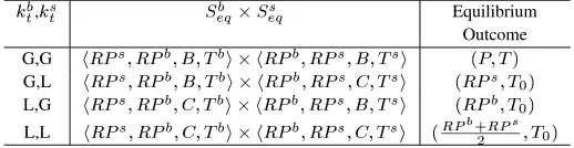
[image:3.612.315.574.5.72.2], Equilibrium Outcome G,G G,L L,G L,L
Table 1: Equilibrium strategies and outcomes for different ne-gotiation scenarios.!indicates
and"indicates
.
denotes
if
, and if
. denotes
the earlier deadline and denotes the second time period.
These adjustments involve experimenting with strategies that it has not tried, with the overall aim of switching away from strategies that give low payoffs to strategies that give high payoffs.
Since bargaining involves two agents with different utility func-tions, we treat the population as being composed of two different subpopulations; one representing the buyer and the other represent-ing the seller. In such asymmetric populations, the evolution of strategies in each subpopulation affects the evolution of strategies in the other subpopulation, (i.e., the strategies co-evolve). Thus we study the competitive co-evolution in which thefitness of an individual in one population is based on direct competition with individuals of the other population.
We represent an agent’sfitness with its utility function and apply the three standard operations ofselection,crossover, andmutation. An agent’s strategy was defined in Section 2 as a tuple of four ele-ments, viz., the initial price, thefinal price, the negotiation decision function and the deadline. Each individual is represented as a string offixed length. The bits of the string (the genes) represent the four elements of an agent’s strategy. The range of values for these genes are as follows. Since each agent knows its opponent’s reservation price (see information state of an agent defined in Section 3), wefix
to be . This is because agreement can never take place
outside the zone of agreement. Thefinal price lies in the range
(i.e.,). The NDF can be anywhere between an
ex-treme Boulware and an exex-treme Conceder for both the agents. The last element is the time at which thefinal price is offered. Since each agent knows its own deadline, wefix the last element of the strategy at the agent’s deadline. In other words, thefirst and the last elements of the strategy arefixed and do not change. For these two
fixed values2, the GA needs tofind the most effective strategy by
varying the and the NDF. (i.e., the second and third elements
of the strategy tuple).
The different stages in an iteration of the GA are as follows. In-dividuals in the two subpopulations are initialised with some strate-gies. How the two populations are initialised is explained in Sec-tion 5. Once initialised, the parent agents in one of the populaSec-tions, say the buyer population, start the negotiation process. Thefi t-ness of the parent agents in both the populations is determined by competition between the agents in the two populations. Each agent competes against all the agents in the other population. The average utility obtained in these negotiations is then used as the agent’sfi t-ness value. In the next stage, offspring agents are created for each
Although thefirst and last elements of the strategy tuple could be
treated as search parameters, we treated them as constants in order to reduce the search space. Note that this encoding includes all possible feasible agreements in the search space, and excludes only that part of the search space where an agreement can never take place (i.e., points outsideor beyond the deadline). Consequently
Tb Ts Tb Ts Tb Ts
1
O
O O
O O
2
3
7 6 5
O
RP
s
RP
b
Ss1
Ss
2 S3s
Sb1
Sb2
S3b
Sb1
Sb2 Sb3
1
Sb
Sb
2 S
b 3
4
O
(a) (b) (c)
[image:4.612.132.480.11.109.2]Time Price Price Price
Figure 3: Possible buyer and seller strategies when
and
.
population using the standard operations of selection, crossover, and mutation. Each of these operations is explained below.
The buyer and seller population size were each set to#.
Se-lection was carried out using thefitness proportionate selection method [10], where individuals are chosen with a probability pro-portional to theirfitness. To perform crossover within a population, we select two individuals randomly. Two crossover points are then chosen randomly and sorted in ascending order. Then the genes between the successive crossover points are alternately exchanged between the individuals with probability. Mutation is the
pro-cess of creating completely new strategies that are not present in the initial population. To perform mutation, a gene (in our case, the second or the third element of the strategy tuple) is selected ran-domly, and a random value is chosen for it from the domain of the gene. We perform mutation on the second and third elements of the strategy tuple because an optimal value needs to be found for these two elements. The mutation rate was. We determined the
sta-ble outcome for different values of#, , and
in the ranges 20
to 75, 0.1 to 0.9, and 0.005 to 0.05 respectively. Increasing the pop-ulation size beyond 50 did not change the stable outcome but only increased the time to stabilize. The stable outcome was, on an av-erage, found to be closest to the equilibrium outcome for ,
and .
To indicate thatfitness proportionate selection is a reasonable method in this case, we carried out the above set of experiments using the other common selection method, namely tournament se-lection [10] with a tournament size of 2. Between the two selec-tion methods, the stable outcome generated byfitness proportion-ate selection was, on average, found to be closer to the equilibrium outcome. Section 5 therefore describes the evolutionary experi-ments for thefitness proportionate selection method for# , , and .
Note that all genetic operations are carried out within a subpop-ulation, i.e., there is no transfer of strategies across the two sub-populations. The simulations stop when the population is stable, i.e.,of the individuals in each subpopulation have the same fitness, for 10 successive generations. This is because, depending on the initialization of the subpopulations, all the individuals in one or both of the subpopulations can have the samefitness values in thefirst iteration itself.
5. THE EVOLUTIONARY EXPERIMENTS
This section determines the stable outcomes and shows how the initial population affects these outcomes. As mentioned in Sec-tion 2, the deadlines are different for and. Let
denote the
agent with the longer deadline andthe one with the shorter
deadline. Let$ and
$
denote the corresponding
popula-tions. To determine if the stable outcome depends on the initial
population, we ran the GA for the following different initial popu-lations for each of the four possible negotiation scenarios listed in Table 1.
Both$
and
$
are initialised to the game-theoretic
equilibrium strategies given in Section 3.
One of the populations is initialised to the equilibrium
strat-egy and the other to some random non-equilibrium strategies.
Both$and$are initialised to some random
non-equilibrium strategies.
5.1 Both buyer and seller prefer a late
agree-ment (
and
)
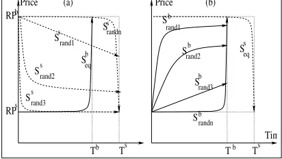
The stable state for each of the three initializations is explained be-low. When all the individuals in each subpopulation are initialised to their respective equilibrium strategies (i.e.,), the stable
out-come was identical to the game-theoretic equilibrium outout-come. As seen in Section 3, in the equilibrium outcome for this scenario, the entire price-surplus goes to the agent with the longer dead-line. This evolutionary behavior can be explained by examining how the strategies in the two subpopulations co-evolve. Consider
$
(which represents the buyer)first. Since all the
individu-als in $
are initialised to the equilibrium strategy (see
Fig-ure 4(a)), they all have the same averagefitness values after the
first round of negotiations. The other population, i.e., $ , is
also initialised to its equilibrium strategy, which gives all its in-dividuals the same averagefitness values after thefirst round of negotiations. The new non-equilibrium strategies that get intro-duced in$
, due to mutation
3, either have a lower value for
than the in
, or an NDF that differs from the NDF in
. These strategies mostly conflict with the vast majority of
equi-librium strategies of$
(the non-equilibrium strategies that are
subsequently introduced into$form a very small fraction of
the entire population), resulting in relatively inferiorfitness values, and eventually dying out, while the equilibrium strategies, being superior, survive to future generations. Turning now to$, the
new non-equilibrium strategies that are generated in$ have a
higher value forthan thein
. In addition, the NDF can
be linear, Boulware or Conceder. Those strategies that use a Con-ceder or linear NDF result in agreement at a lower price, yield a
fitness value that is lower than the equilibrium strategyfitness, and as a result do not survive. Those non-equilibrium strategies that use the Boulware NDF result in the same outcome as the equilibrium strategies. In other words, even in$
, only those individuals that
RP RP
Tb Ts
Ss
Tb Ts
eq
Srand2b rand3
S Srand1b
b
Sbrand4
Sbrand5 b
s
eq
Sb
eq
Ss
Time
[image:5.612.333.539.8.124.2]Price (a) Price (b)
Figure 4: Buyer and seller population initialization.
play the equilibrium strategy reach the stable state. The majority of individuals in both the populations continue to play their respective equilibrium strategies. The stable outcome is therefore identical to the game-theoretic equilibrium outcome.
For the second initialization, the stable outcome was found
to depend on the initial population corresponding to the agent with the earlier deadline. There are two possibilities for
. Either $
is initialised randomly and
$
with its equilibrium
strat-egy, or$is initialised with its equilibrium strategy and$
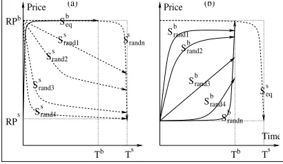
randomly. Each of these is explained below. When$ is
ini-tialised with the equilibrium strategy and$
is initialised
ran-domly, both the populations stabilised at the equilibrium strategies. To understand this, consider$. The initial populations for
this scenario are depicted in Figure 5(a). Since all the individu-als in$ play the same strategy, they all have the samefi
t-ness values. The new strategies that are generated from mutation are non-equilibrium strategies. The individuals that play the equi-librium strategy have a higherfitness than those playing the non-equilibrium strategy. The new strategies introduced from mutation thus get eliminated, while the equilibrium strategy prevails. The other population, i.e.,$
, is initialised randomly, resulting in a
differentfitness value to each individual. The closer the strategy is to the equilibrium strategy, the higher itsfitness. The close-to-equilibrium strategies thusflourish in$
at the expense of the
non-equilibrium strategies. The behavior of$adapts to best
suit the predominantly equilibrium strategy of$ .
$ ’s best
reply to$
is the equilibrium strategy. Thus
$
dynamically
changes its strategy and stabilizes at the equilibrium strategy. Both populations thus stabilize at the equilibrium strategy.
For
, when$
was initialised randomly, the stable
out-come was found to be different from the equilibrium outout-come. The agent with the earlier deadline obtains a higher utility than its util-ity from the equilibrium outcome. But the agent with the longer deadline gets a lower than equilibrium utility. This is explained as follows. Consider$first, which is initialised to the equilibrium
strategy. The equilibrium strategy of$
conflicts with most of
the strategies of$
, since they are non-equilibrium (see
Fig-ure 5(b)). Moreover, since all individuals play the same strategy, thefitness values are the same for all of them, and correspond to the conflict outcome. The new strategies that are generated from mu-tation, although being non-equilibrium strategies, result in agree-ment and are therebyfitter than the equilibrium strategies (recall that an agreement always gives an agent a higher utility than its conflict utility). The number of non-equilibrium strategies thus in-creases from one generation to the next. But the rate of this change is very slow, since most of the individuals play the equilibrium strategy. The chances that two strategies selected for crossover are
b
s Srand3 s
Srand2s
Ssrand1 S
s randn
Sbeq
Tb Ts
rand1
Sb
rand2
Sb
rand3
Sb
Seqs
Srandnb
Tb Ts
RP
RP
Price (a) Price (b)
Tim
Figure 5: Buyer and seller population initialization.
identical is high. Crossover between two identical strategies yields the same strategy. Thus while mutation can yield a new strategy, the chance of generating new strategies through crossover is low.
$
thus has a very low rate of change. The other population, $, is initialised randomly but thefitness levels of the
individ-uals in this population too are equal, and correspond to the
con-flict outcome. However, as non-equilibrium strategies get gener-ated in$, the individuals in$have differentfitness levels
since they play random strategies. Since all individuals play differ-ent strategies, the rate of evolution of$
is faster than
$
.
Eventually, $
evolves towards a strategy that differs slightly
from the equilibrium strategy, since only such strategies result in a better agreement with the non-equilibrium strategies of$
,
and yield a higher payoff than the conflict outcome. On the other hand, $evolves towards a strategy that is the best reply to
this non-equilibrium strategy of$
. Both populations thus shift
away from the initial conflict outcome and eventually stabilize at a non-equilibrium one.
For initialization
, where both$ and
$
are initialised
randomly, the stable state was again different from the theoretical equilibrium outcome. It was also different from the stable state for the case where$
was initialised randomly and $
with its
equilibrium strategy.
The experiments for each of the initialisations,, andwere
repeated 50 times. Despite the presence of randomness, we found that the outcomes in these different runs did not vary by more than
and the relationship between the outcomes for,, and
always remained the same. These results (averaged over all the runs) are summarised in Table 2. For all the runs, was 100,
was 20, and
were both greater than 0,
was 90, and
was 195. As seen in the table, an agreement is always reached at the earlier deadline (i.e.,
). The price of agreement lies
between
and
and is close to
, the reservation price of the agent with the earlier deadline.
Table 2 also shows that the dominant strategy for
(which
represents the buyer) is to initialize the population randomly since this results in agreement at a lower price. The dominant strategy for
(which represents the seller) is to initialize all the individuals
with its equilibrium strategy. Note that andhave similar time
preferences. The time of agreement in all cases was the earlier deadline, which gives the maximum possible utility from time to both the agents. The price of agreement favours
.
[image:5.612.72.276.9.123.2]Equilibrium Strategy Random Eq. Strategy (100,90) (100,90) Random (95,90) (80,90)
Table 2: Stable outcomes for different initialisations. Rows in-dicate and columns indicate. Thefirst entry in each pair
denotes the price, and the second entry the time of agreement.
5.2 Both buyer and seller prefer an early
agree-ment (
and
)
The set of experiments described above was repeated for the case where both andlose utility on time. The stable outcome was
the same as the equilibrium outcome, irrespective of whether the two subpopulations were initialised with the equilibrium strategy or randomly. This is explained below. Consider the case where both
$ and
$
are initialised with their respective equilibrium
strategies (i.e.,). All the individuals have the samefitness levels,
and new strategies that get generated from mutation, being rela-tively inferior, do not reach the stable state. The stable outcome is therefore the same as the equilibrium outcome. The situation where
$
is initialised randomly and
$
is initialised with its
equi-librium strategy (i.e.,
) is depicted in Figure 4(b). As seen in the figure, all the interactions initially result in an agreement. More-over, thefitness level of all the individuals in$
is the same,
since they all play the equilibrium strategy. The new strategies that are generated by means of mutation, being inferior to the equilib-rium strategy, get eliminated. This is because the constant
in our
utility function is greater than the constant
(see Section 2 for the
definition of utility function which is used as an individualsfitness). On the other hand, the individuals in$have differentfitness
values, as they all play different random strategies. The closer a strategy to the equilibrium strategy, the higher itsfitness. $
thus evolves to its equilibrium strategy. Both the subpopulations thus stabilize at their respective equilibrium strategies and result in a stable outcome that is identical to the equilibrium outcome.
When$is initialised with the equilibrium strategy and$
is initialised randomly, the stable outcome was the same as the equilibrium outcome. As in the previous case, all the interactions initially result in an agreement but,$remains stable at the
equilibrium strategy, while$evolves towards its equilibrium
strategy. This co-evolution of strategies eventually results in the same stable outcome as the equilibrium outcome.
Finally, when both $ and $ are initialised randomly
(i.e.,
), both populations stabilized at the game-theoretic
equi-librium strategy. To sum up, when
and
, the stable outcome always
matched the equilibrium outcome.
5.3 Buyer prefers an early agreement and seller
prefers a late one (
and
)
When both$ and
$
are initialised to their respective
equi-librium strategies (i.e.,), as in the previous two subsections, the
stable outcome was the same as the equilibrium outcome. For ,
when$
is initialised randomly and
$
with its equilibrium
strategy, then the stable outcome was the same as the equilibrium outcome. In the initial populations depicted in Figure 6(b), thefirst round of negotiations mostly result in conflict between the equilib-rium strategy of$
and the random strategies of
$
.
More-over, almost all the individuals in both the populations have the samefitness value, which is equal to the conflict utility. In the next generation, the new strategies that are generated through mutation
RP
RP
Ts
Tb Tb Ts
Sbeq
S S
S
S
s s
s
s
Ssrandn
rand4 rand3
rand2 rand1
Sseq
S S
S
S S
b b
b
b b rand1
rand2
rand3
rand4 randn s
(a) (b)
b
Time Price
[image:6.612.333.538.6.125.2]Price
Figure 6: Buyer and seller population initialization when
and
.
in$
, have a different NDF. They are either less Boulware,
lin-ear, or Conceder and result in agreement with some or all of the strategies of$
. However the majority of the individuals still
play the equilibrium strategy, and thereby have the samefitness.
$thus evolves slowly. Looking at$ we see that, since
all individuals play a different strategy, it evolves relatively faster than$
. This is because new strategies are generated in
$
through two operations (viz., crossover and mutation) as opposed to the generation of new strategies in$
through mutation alone.
In other words, as$
evolves faster, it moves towards the
strat-egy that is the most effective reply to the predominantly equilibrium strategy played by$. Eventually,$stabilizes at its
equi-librium strategy and$
stabilizes at a strategy that is slightly less
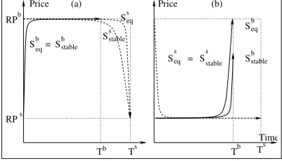
Boulware than its equilibrium strategy. The stable and equilibrium strategies for (
,
) are depicted in Figure 8(a). As seen
in thefigure, although the stable strategy of$
is not the same
as the equilibrium strategy, agreement is still reached at the same point as the equilibrium outcome. This is because the difference in price between the two strategies (
and
), is high at ,
and almost zero near the beginning of negotiation. Since$
stabilises at its equilibrium strategy, which uses the Conceder func-tion, the stable outcome results in agreement near the beginning of negotiation and is the same as the equilibrium outcome. Contrast this with the stable outcome corresponding to Figure 5(b), where
. Since agreement takes place at
, the stable outcome
dif-fers from the equilibrium outcome. But in Figure 8(a),
, and
the stable agreement takes place at the beginning of negotiation, which is identical to the equilibrium outcome.
For , when
$
is initialised randomly and
$
with its
equilibrium strategy (see Figure 6(a)), the outcome was again the same as the equilibrium outcome. Notice that in this case, initially all the interactions result in agreement since$
plays the
equi-librium strategy (i.e., the Conceder NDF). All the individuals in
$therefore have the samefitness values. On the other hand,
the individuals in$
have differentfitness values.
$
evolves
faster than$
, and stabilizes at a strategy that is the best reply
to the equilibrium strategy played by$. The new strategies
that get introduced in$
, through mutation, being inferior to
its equilibrium strategy, do not survive. Both the populations there-fore stabilise at their respective equilibrium strategies, and result in equilibrium outcome.
When both$ and
$
are initialised randomly (i.e.,
), the
stable outcome was again found to be the same as the equilibrium outcome. Thus, irrespective of the initialization (,, or) of
Price
RP
Time
(a) (b)
RP
Ts
Tb Tb Ts
Price
s b
S S S
S
S S
s rand1 s
rand2
s rand3
s rand4 s randn
b
eq S
S
S
S
b b
b
b
Sseq randn
[image:7.612.70.277.6.125.2]Sbrand4 rand3 rand2 rand1
Figure 7: Buyer and seller population initialization when
and
.
5.4 Buyer prefers a late agreement and seller
prefers an early one (
and
)
We begin with, the case where both$ and
$
are
ini-tialised to their respective equilibrium strategies. As in the previous subsections, the stable outcome was the same as the equilibrium outcome. For
, when
$
is initialised randomly and $
is initialised with its equilibrium strategy, the stable outcome was the same as the equilibrium outcome. Figure 7(b) shows the initial populations for this scenario. As seen in thefigure, all the inter-actions result in agreement. Moreover, since all the individuals in
$play the equilibrium strategy, they all have the samefitness.
The new strategies that are generated through mutation, being infe-rior to the equilibrium strategy, get eliminated. On the other hand, the individuals in$play random strategies and have different fitness values.$
thus evolves faster than $
, and stabilizes
at a strategy that is the best reply to the equilibrium strategy played by$. The best reply to$is’s equilibrium strategy. Both
populations thus stabilize at their respective equilibrium strategies. The stable outcome therefore matches the equilibrium outcome.
For, when$is initialised with the equilibrium strategy
and$
is initialised randomly, the stable outcome was again the
same as the equilibrium outcome. As shown in Figure 7(a), all the initial interactions between the two populations result in agree-ment. Furthermore, since$
is initialised with the equilibrium
strategy, all its individuals have the samefitness values, while the individuals in$ have differentfitness values as they are
ini-tialised randomly. Within$
, the closer an individual’s strategy
is to the equilibrium strategy, the higher itsfitness is, since it is the best reply to the equilibrium strategy played by all the individuals of$. $ therefore evolves faster than$ and
stabi-lizes at its equilibrium strategy. On the other hand, the new non-equilibrium strategies that are generated in$
, through
mu-tation, have an inferiorfitness relative to the equilibrium strategy, and thereby get eliminated. Thus$
and
$
both stabilize at
their respective equilibrium strategies, and result in the equilibrium outcome.
Finally, when both $ and
$
are initialised randomly
(i.e.,
), the stable outcome was again found to be the same as
the equilibrium outcome. $
stabilized at the non-equilibrium
strategy. In the stable strategy of$all the elements except the
second, (i.e., thefinal price) were the same as the elements in the equilibrium strategy. Although thefinal price in the stable strategy was less than , it resulted in the equilibrium outcome since
the, the NDF and the deadline were the same as in (see
Figure 8(b)).
RP
RP
Ts Tb b
eq
Seq
Ss
s
stable
Sseq
Sbeq
Sbstable b
s
S =Sbstable
= Ssstable
Tb Ts
Price (a) Price (b)
Time
Figure 8: Stable vs. equilibrium strategies. (a)
and
(b)
and
.
5.5 A summary of key results
The above analysis leads to two main conclusions. Firstly, al-though game-theoretically each agent has a dominant strategy, the results of our analysis show that when the population is asymmetric and the strategies in the two populations co-evolve, the stable out-come of the evolutionary approach does not always coincide with the game-theoretic equilibrium outcome. Secondly, as the play-ers mutually adapt to each other’s strategy, the stable outcome de-pends on the initial population. More specifically, when
and
, the outcomes of these two approaches differ. As seen
in Table 2, the dominant strategy for(which in our case
repre-sents the buyer) is to initialize the population randomly since this results in agreement at a lower price. The dominant strategy for
(which represents the seller) is to initialize all the individuals with its equilibrium strategy. Also, as shown in Table 2, the outcome generated by the evolutionary approach is more in favour of
,
than the equilibrium outcome. The difference however is small. While the equilibrium price of agreement is 100, the price at the stable state (for the right initialization) is 95. For all the remaining scenarios (i.e.,
for at least one of the agents) the
game-theoretic equilibrium outcome matches the stable outcome of the evolutionary model, irrespective of how the two populations are initialised (i.e.,,, or).
From thesefindings it is clear that implementing software agents using the game-theoretic approach is computationally simpler (since the equilibrium strategies can be determined on the basis of the agents’ information states). Once they are determined, the agents just need to be coded with these strategies. In contrast, the stable strategies in the evolutionary model depend on how the popula-tions are initialised. However, an agent may not know exactly how the opponent’s population is initialised and, consequently, the GA learning needs to be done online every time there is a negotiation.
6. RELATED RESEARCH
[image:7.612.333.539.7.125.2]two paths yield the same payoff for one of the players). However, all these models are based on the assumption that agents are drawn from a single population, in which all the individuals have the same utility function. In a more realistic bargaining scenario, the buyer and the seller have different utility functions. We therefore treat the population as being asymmetric, i.e., the population is com-posed of two separate subpopulations - one representing the buyer and the other representing the seller since they have different util-ity functions. Our work thus considers competitive co-evolution, in whichfitness is based on direct competition between individu-als selected from two independently evolving populations of buyers and sellers. Moreover, we also show that when the two subpopu-lations co-evolve, then the stable outcome depends on how the two subpopulations are initialised.
Matos et al [9] use GAs to analyse multi-issue negotiation. The population comprises of two subpopulations; one representing the buyer and other representing the seller. They use afitness function based on the sum of the score across all the competitions. The and populations evolve simultaneously. In real-life bargaining
situations each participant tries to maximize its own utility and not the sum of the participants’ utilities. We therefore consider two asymmetric subpopulations in which the strategies co-evolve.
In summary, existing evolutionary models study the bargaining behavior of agents either for a symmetric population (i.e., they as-sume that both the parties in a game have the same utility function) or study the simultaneous evolution of strategies if the population is asymmetric, by focussing on a specific negotiation scenario. Our work differs from existing models in the following ways. Firstly, we consider an asymmetric population and study the competitive co-evolution of strategies in the two subpopulations. The second difference lies in the stable outcomes generated by the evolutionary models for symmetric and asymmetric populations. For symmetric games of simultaneous offers it has been shown that the evolution-ary equilibrium coincides with the Nash equilibrium [17], while for symmetric games of alternating offers the evolutionarily stable outcome are close to the game-theoretic equilibrium under certain conditions [1]. In contrast to this, our study shows that, if the popu-lation is asymmetric, the stable outcome of the evolutionary model can differ from the game-theoretic outcome even when each agent has a dominant strategy at every period at which it makes a move. Furthermore, our study also highlights the effect of the initial pop-ulation on the stable state.
7. CONCLUSIONS AND FUTURE WORK
This paper studied the bargaining behavior of boundedly rational agents using GAs and compared the results with the game-theoretic equilibrium outcome, for a particular model of negotiation based on negotiation decision functions. In this negotiation game of incom-plete information, each agent has a unique strategy that is domi-nant at every information state at which it makes a move. In the evolutionary counterpart of this model, there is a competitive co-evolution of strategies between two asymmetric populations. Each player learns the most effective strategy that is the best reply to the opponent’s strategy. The key conclusion of our analysis is that although the agents in the game-theoretic model have dominant strategies, the stable state of the corresponding evolutionary model does not always match the equilibrium outcome. Furthermore, as the players mutually adapt to each other’s strategy, the stable out-come depends on the initial population.
Our present work used genetic algorithm learning to study the bargaining behavior of boundedly rational agents. In order to get more general results, it would be interesting to extend the analysis to other learning mechanisms.
Acknowledgements
This research was supported by the EPSRC under grant GR/M07052.
8. REFERENCES
[1] K. Binmore, M. Piccione, and L. Samuelson. Evolutionary stability in alternating-offers bargaining games.Journal of Economic Theory, 80:257–291, 1998.
[2] K. Binmore and L. Samuelson. Evolution and mixed strategies.Games and Economic Behavior, 34:200–226, 2001.
[3] R. Cressman and K. H. Schlag. The dynamic (in)stability of backwards induction.Journal of Economic Theory, 83:260–285, 1998.
[4] T. Ellingsen. The evolution of bargaining behavior.The Quarterly Journal of Economics, pages 581–602, May 1997. [5] P. Faratin, C. Sierra, and N. R. Jennings. Negotiation
decision functions for autonomous agents.International Journal of Robotics and Autonomous Systems,
24(3-4):159–182, 1998.
[6] S. S. Fatima, M. Wooldridge, and N. R. Jennings. An agenda based framework for multi-issue negotiation.Artificial Intelligence Journal (to appear).
[7] S. S. Fatima, M. Wooldridge, and N. R. Jennings. The influence of information on negotiation equilibrium. In J. Padget, O. Shehory, D. Parkes, N. Sadeh, and W. E. Walsh, editors,Agent Mediated Electronic Commerce IV Designing Mechanisms and Systems, pages 180–193. Springer Verlag LNAI-2531, 2002.
[8] S. S. Fatima, M. Wooldridge, and N. R. Jennings. Multi-issue negotiation under time constraints. In
Proceedings of the First International Conference on Autonomous Agents and Multi-Agent Systems (AAMAS-02), pages 143–150, Bologna, Italy, 2002.
[9] N. Matos, C. Sierra, and N. R. Jennings. Determining successful negotiation startegies: An evolutionary approach. InProceedings of the 3rd International Conference on Multi-Agent Systems (ICMAS-98), pages 182–189, 1998. [10] M. Mitchell.An Introduction to Genetic Algorithms. The
MIT Press, Cambridge, Massachusetts, 2001.
[11] H. Raiffa.The Art and Science of Negotiation. Harvard University Press, Cambridge, USA, 1982.
[12] A. E. Roth. Bargaining experiments. In J. Kagel and A. E. Roth, editors,Handbook of Experimental Economics. Princeton NJ, Princeton University Press, 1995.
[13] A. Rubinstein. Perfect equilibrium in a bargaining model.
Econometrica, 50(1):97–109, January 1982. [14] A. Rubinstein. A bargaining model with incomplete
information about time preferences.Econometrica, 53:1151–1172, January 1985.
[15] T. Sandholm and N. Vulkan. Bargaining with deadlines. In
AAAI-99, pages 44–51, Orlando, FL, 1999.
[16] J. M. Smith.Evolution and the theory of games. Cambridge University Press, Cambridge, 1982.
[17] J. W. Weibull.Evolutionary game theory. MIT Press, 1997. [18] H. P. Young. An evolutionary model of bargaining.Journal