Consistent estimation in the bilinear multivariate errors in variables model

>Springer-Verlag 2003

Consistent estimation in the bilinear multivariate

errors-in-variables model

A. Kukush1, I. Markovsky1, S. Van Hu¤el1

ESAT, SCD-SISTA, K.U. Leuven, Kasteelpark 10, B-3001 Leuven-Heverlee, Belgium (e-mail: Sabine.VanHu¤[email protected])

Abstract. A bilinear multivariate errors-in-variables model is considered. It corresponds to an overdetermined set of linear equationsAXB¼C,AA_Rmn_, BARpq, in which the dataA,B, Care perturbed by errors. The total least squares estimator is inconsistent in this case.

An adjusted least squares estimator XX^ is constructed, which converges to the true valueX, as m!y_{, q!}y_{. A small sample modification of the} estimator is presented, which is more stable for smallmandq and is asymp-totically equivalent to the adjusted least squares estimator. The theoretical results are confirmed by a simulation study.

Key words: bilinear multivariate measurement error models, errors-in-variables models, adjusted least squares, consistency, asymptotic normality, small sample modification

1 Introduction

Many linear parameter estimation problems [VV91] can be reduced to solving an overdetermined set of linear equations

AXAB: ð1Þ

computes correction matricesDAandDBof minimal Frobenius norm in order to make the corrected set of equations

ðADAÞX ¼BDB

compatible and has become very popular in engineering since the early eighties due to the existence of computationally attractive algorithms based on the singular value decomposition (SVD) [GV80, VV91].

Since then several generalizations of the TLS estimator have been pre-sented. In particular, we mention the generalized TLS estimator, based on the generalized SVD, which provides consistent estimates ofX provided the measurement errors in ½A B are row-wise i.i.d. with zero mean and same covariance matrix, known up to a factor of proportionality.

In this paper we generalize the linear model in (1) to a bilinear model, represented as

AXBAC ð2Þ

This model can be considered as a special case of a polynomial model, namely a quadratic measurement error model [Ful87, CRS95].

It should be noted that the TLS principle can no longer be applied to model (2) in order to provide consistent estimates. Indeed, as mentioned in [Ful87], adding correction matrices DA, DB and DC of minimal Frobenius norm in order to makeðADAÞXðBDBÞ ¼CDC compatible results in biased estimates for the parameterX. In this paper an adjusted least squares (ALS) estimator [CRS95, CS98] ofXis presented and shown to be consistent. Next we give two examples where the bilinear measurement errors model (2) arises.

Example 1(Total production cost model). Assume that rproduction inputs

(materials, parts, labor, etc.) are combined to makenproducts. Letbk be the

price per unit of thek-th production input and xjk be the number of units of

thek-th production input, required to produce one unit of the j-th product.

The production costs per unit of the j-th product is the j-th element of the vector

y¼Xb:

Letajbe a required quantity to be produced of the j-th product. The total

quantity of thek-th production input needed is thek-th element of the vector z¼XTa:

The total production cost c is zT_{b, which gives a ‘‘single measurement’’}

AXB¼Cmodel aTXb¼c:

and (approximate) total costs cil_{, corresponding to all combinations of the}

given quantities to be produced and prices. Then the model is ða1_ÞT

.. .

ðam_ÞT

2 6 6 4

3 7 7 5

|fflfflfflfflfflffl{zfflfflfflfflfflffl}

A

X½b1. . .bq |fflfflfflfflfflffl{zfflfflfflfflfflffl}

B

¼

c11 c1q .. .

.. .

cm1 cmq 2

6 4

3 7 5

|fflfflfflfflfflfflfflfflfflfflffl{zfflfflfflfflfflfflfflfflfflfflffl}

C :

Estimation ofxjk in the modelAXB¼C, can be interpreted as: estimate

the number of units of thek-th production input, required to produce one unit of the j-th product.

Example 2(Estimation of the fundamental matrix [MM98]). Two images are

captured by a mobile camera andmmatching pixels are located. Let

ui¼

uið1Þ

uið2Þ

1 2 6 4

3 7

5 and vi¼

við1Þ

við2Þ

1 2 6 4

3 7

5; i¼1;. . .;m

represent the homogeneous pixel coordinates in the first and second image respectively. The so calledepipolar constraintrelates the corresponding pixel coordinates by the model

v_iTFui¼0; i¼1;. . .;N; ð3Þ

where FAR33, rankðFÞ ¼2 is the fundamental matrix which is identical for all pairs of corresponding vectorsui,vi, 1aiaN. Estimation ofFfrom

the given noisy data is calledstructure from motion problem and is a central problem in computer vision.

In [KMV01] we modified the adjusted least squares estimator derived in this paper for the model (3).

The notation we use is standard. For any matrixT,tij denotes thei;j-th

element ofT. The bold symbol Edenotes mathematical expectation. It acts on the expression on the right up to an addition or subtraction sign. Condi-tional expectation of x, conditioned on C, is denoted by E½xjC. The nota-tion covðxÞdenotes the covariance matrixExTxExTExandAydenotes the pseudo-inverse ofA. In the formulas ‘‘const’’ denotesany constant value (for example, we can write const2 ¼const).

2 The model

We consider the model

AXB¼C: ð4Þ

Here AARmn, BARpq, CARmq are observations and XARnp is a

parameterof interest. We suppose that

A¼A0þAA~; B¼B0þBB~; C¼C0þCC~; ð5Þ

and that there existsX0ARnp such that A0X0B0¼C0:

HereA0,B0, andC0 arenominalortrue values andAA,~ BB, and~ CC~areerrors.

The matrixX0 is the nominal or true value of the parameter. From the point

of view of errors-in-variables models,CC~represents theequation error, whileAA~ andBB~represent themeasurement errors.

Looking for asymptotic results in the estimation ofXin the model (4), we fix the dimensions ofX,nand p, and let the number of measurements,mand

q, increase. The measurements are represented by the rows ofA, the columns

ofBand the elements ofC. For the whole paper we denote V_AA~vEAA~TAA~; V_BB~vEBB~BB~T:

The matrices V_AA~and V_BB~ are supposed to be known, while the variances of the

entries ofCC are unknown.~

Specific notation is set in the course of exposition. The assumptions used in the paper are enumerated. Global assumption for the paper is assumption (i). (i). The errors f~aaij;ib1;1ajang, fbb~kl;1akap;lb1g and fcc~il;ib1,

lb1gform three independent arrays of r.v., which are centered and pos-sess finite second order moments.

More assumptions are stated where necessary.

The model (4–5) is a bilinear regression measurement error model. In a scalar form it can be written as

cil¼

X

j;k

~ a

a0_ijxjkbb~kl0 þcc~il; 1aiam;1alaq;

aij¼a0ijþaa~ij; 1aiam;1ajan;

bkl¼b0klþbb~kl; 1akap;1alaq:

ð6Þ

Here the design points a0

ij and b0kl are unobservable non-stochastic variables

and the true valuec0

il is a nonlinear function ofA0andB0.

The model (6) is a particular case of a quadratic model; it is bilinear with respect to the compound nuisance parameters½A0 B0. For polynomial

errors-in-variables models an ALS estimator is proposed in [CS98]. It is consistent. In [CRS95, Chapter 6], the method of corrected score functions is presented and in [Bar00] it is mentioned that an ALS estimator in a polynomial model is generated by the method of corrected score functions.

3 The score equation and an ALS estimator

We start with the LS objective function

qlsðX;A;B;CÞvkAXBCk

2

F: ð7Þ

In the space of matricesRnp, we introduce a scalar product h_T;Siv_trðTST_Þ; T;SA_Rnp:

The derivativeqqls=qX is a linear functional on Rnp. It acts on H ARnp according to the rule

1 2

qqls

qX ðHÞ ¼trððAXBCÞðAHBÞ

T_{Þ ¼trðA}T_ðAXBCÞBT_HT_Þ

¼h_AT_ðAXBCÞBT;Hi: ð8Þ

We can identify the derivativeqqls=qX with a matrix, which represents it in

the equality (8). Thus it is redefined as 1

2

qqls

qX ¼ ðA

T_AÞXðBBT_{Þ A}T_CBT_:

In the absence of measurement errors, i.e. whenAA~¼0 andBB~¼0, see (5), the LS estimator is obtained by minimizing (7) or (what is asymptotically equiv-alent) via the score equation1

2qqls=qX ¼0. Thus the score function for the LS

method is

clsðX;A;B;CÞvðA

T_AÞXðBBT_{Þ A}T_CBT_;

and the LS estimator is consistent in the absence of measurement errors. Now, we are looking for a corrected score functionc, such that

E½cðX;A0þAA~;B0þBB~;CÞ jC ¼clsðX;A0;B0;CÞ for allX;A0;B0;C:

We seekcin the formc¼clsc₁. We have by assumption (i)

E½clsðX;A0þAA~;B0þBB~;CÞ jC

¼clsðX;A0;B0;CÞ þEAA~ T_AAXB~

0BT0 þEA T

0A0XBB~BB~TþV_AA~XV_BB~

with

c₁₁ðB0ÞvV_AA~XB0BT0;

c₁₂ðA0ÞvAT0A0XV_BB~:

To find a proper correction termc1 we consider Ec₁₁ðB0þBBÞ ¼~ V_AA~XB0BT0 þV_AA~XV_BB~;

Ec₁₂ðA0þAAÞ ¼~ AT0A0XV_BB~þV_AA~XV_BB~:

ð9Þ

Therefore

c1ðA;BÞ ¼c11ðBÞ þc12ðAÞ V_AA~XV_BB~

and

cðX;A;B;CÞ

¼ ðATAÞXðBBTÞ ATCBTV_AA~XðBBTÞ ðATAÞXV_BB~þV_AA~XV_BB~

¼ ðATAV_AA~ÞXðBBTV_BB~Þ ATCBT:

The ALS estimatorXX^ is defined from the equation

cðX;A;B;CÞ ¼0: ð10Þ

As an estimator we can take ^

X

Xv_ðATAV_AA~ÞyðATCBTÞðBBTV_BB~Þy: ð11Þ

IfAT_AV ~ A

AandBBTVBB~are non-singular, then (11) satisfies (10). Later on

we shall show that these matrices are non-singular with probability tending to one as the number of measurements (rows ofAand columns ofB) is tending to infinity. Observe that (11) reduces to the generalized TLS estimator [VV89, Gal82], in the caseB¼Ip,BB~¼0 under the assumption (i).

4 Weak and strong consistency

We introduce further assumptions.

(ii). The rows of AA~are independent, i.e. ð~aaij;i1;1ajanÞ are

indepen-dent, the columns of BB~ are independent, i.e. ðbb~kl;1akap;lb1Þ are

independent, and all elements ofCC~are independent, i.e.ðcc~il;ib1;lb1Þ

are independent. (iii). Eaa~4

ijaconst,Ebb~4klaconst, andE~ccil2aconst.

(iv). We denote

and assume that

lmaxðVA0Þ þm

l2_minðVA0Þ

!0 asm!y; and lmaxðVB0Þ þq

l2_minðVB0Þ

!0 asq!y:

The assumption (iv) corresponds to the condition of weak consistency, given in [Gal82] for the maximum likelihood estimator in the model (1).

Theorem 1 (Weak consistency). Assume that assumptions (i) to (iv) hold.

Then the estimatorXX given in (11) converges to X^ 0in probability, as m!y

and q!y.

Proof.Denote

UAvATAV_AA~; UBvBBTV_BB~: ð12Þ

By assumption (iv),VA0 is non-singular formbm0 andVB0 is non-singular

forqbq0for some fixedm0andq0. Formbm0,qbq0, we rewrite equation

(10) in the form

V_A01UAXUBVB01¼VA01ðATA0X0B0BTþATCBC~ TÞVB01: ð13Þ

For consistency, it is enough to show that V_A01UA!

p

In and UBVB01 !

p

Ip; ð14Þ

V_A01ðAT_A 0Þ !

p

In and B0B0TV

1 B0 !

p

Ip; ð15Þ

V_A01ATCCB~ TV_B01!p 0: ð16Þ

The proofs of (14)–(16) are given in the Appendix. r

The main probabilistic tool to prove the strong consistency is the following matrix analogue of the Rosenthal inequality, see [Ros70].

Lemma 1.Letfhi;ib1gbe a sequence of independent r.v.,Ehi¼0, i¼1;2;. . .

Then for any real number tb2, and for all mb1

EX

m

i¼1

h_i

t

acðtÞmax X

m

i¼1

Ejh_ijt; X m

i¼1 Eh_i2

!t=2

0 @

1 A;

where cðtÞdepends on t, but it does not depend on m.

We strengthen assumptions (iii) and (iv).

(v). For fixed real number rb2, Ejaa~ijj2raconst, Ejbb~klj2raconst, and Ej~ccilj2raconst.

(vi). For fixedm0b1,

Xy

m¼m0

mr=2

l_minr ðVA0Þ

þl

r maxðVA0Þ

l2r_minðVA0Þ

!

and for fixedq0b1

Xy

q¼q0

qr=2

lr_minðVB0Þ

þl

r maxðVB0Þ

l2r_minðVB0Þ

!

<y;

whereris defined in assumption (v).

Theorem 2 (Strong consistency). Assume that assumptions (i), (ii), (v) and

(vi) hold. Then the estimatorXX given in (11) converges to X^ 0 a.s., as m!y,

q!y_.

Proof.See Appendix.

5 Rate of convergence

Let the assumptions of Theorem 1 hold. With probability tending to 1 we have

ðAT_AV ~ A

AÞXXðBB^ TV_BB~Þ ¼ATCBT: ð17Þ

We setXX^vX0þDD^and considermbm0,qbq0, for whichVA0 andVB0 are

non-singular. From (17) we have

ðATAV_AA~ÞDD^ðBBTV_BB~Þ ¼ATðA0X0B0þCCÞB~ T

ðAT_AV ~ A AÞX0ðBB

T_V ~ B

BÞ: ð18Þ

Using the notations (12) we have

V_A01UADD^UBVB01¼VA01ATCBC~ TVB01þVA01ðATA0X0B0BT

ðAT_AV ~ A

AÞX0ðBBTV_BB~ÞÞV_B01vR1þR2: ð19Þ

By (14), the LHS of (19) equals

LHS¼ ðInþopð1ÞÞDD^ðIpþopð1ÞÞ ð20Þ

Next, see Section 4,

R1¼VA01ATCCB~ TVB01

¼

ffiffiffiffiffiffiffiffiffiffiffiffiffiffiffiffiffiffiffiffiffiffiffiffiffiffiffiffiffi

lmaxðVA0Þ þm

p

lminðVA0Þ

ffiffiffiffiffiffiffiffiffiffiffiffiffiffiffiffiffiffiffiffiffiffiffiffiffiffiffiffiffi

lmaxðVB0Þ þq

p

lminðVb0Þ

Opð1Þ: ð21Þ

R21 ¼VA01ðATA0X0B0BTVA0X0VB0ÞVB01

¼ Inþ

ffiffiffiffiffiffiffiffiffiffiffiffiffiffiffiffiffiffiffiffi

lmaxðVA0Þ

p

lminðVA0Þ

Opð1Þ

!

X0 Ipþ

ffiffiffiffiffiffiffiffiffiffiffiffiffiffiffiffiffiffiffiffi

lmaxðVB0Þ

p

lminðVB0Þ

Opð1Þ

!

X0; ð22Þ

kR21kF ¼

ffiffiffiffiffiffiffiffiffiffiffiffiffiffiffiffiffiffiffiffi

lmaxðVA0Þ

p

lminðVA0Þ

þ

ffiffiffiffiffiffiffiffiffiffiffiffiffiffiffiffiffiffiffiffi

lmaxðVB0Þ

p

lminðVB0Þ

!

Opð1Þ ð23Þ

and

R22 ¼VA01ðATAV_AA~ÞX0ðBBTV_BB~VA0X0VB0ÞVB01

¼ Inþ

ffiffiffiffi m p

þ ffiffiffiffiffiffiffiffiffiffiffiffiffiffiffiffiffiffiffiffilmaxðVA0Þ

p

lminðVA0Þ

Opð1Þ

! X0

Ipþ

ffiffiffi q p

þ ffiffiffiffiffiffiffiffiffiffiffiffiffiffiffiffiffiffiffiffilmaxðVB0Þ

p

lminðVB0Þ

Opð1Þ

!

X0; ð24Þ

kR22kF ¼

ffiffiffiffi m p

þ ffiffiffiffiffiffiffiffiffiffiffiffiffiffiffiffiffiffiffiffilmaxðVA0Þ

p

lminðVA0Þ

þ ffiffiffi q p

þ ffiffiffiffiffiffiffiffiffiffiffiffiffiffiffiffiffiffiffiffilmaxðVB0Þ

p

lminðVB0Þ

!

Opð1Þ: ð25Þ

Therefore from (19), (20), and (21) to (25) we obtain k_XX^_X0k

F ¼ ðumþvqÞOpð1Þ; ð26Þ

where

umv

ffiffiffiffi m p

þ ffiffiffiffiffiffiffiffiffiffiffiffiffiffiffiffiffiffiffiffilmaxðVA0Þ

p

lminðVA0Þ

; vqv

ffiffiffi q p

þ ffiffiffiffiffiffiffiffiffiffiffiffiffiffiffiffiffiffiffiffilmaxðVB0Þ

p

lminðVB0Þ

: ð27Þ

6 Asymptotic normality

6.1 Expansion forDD^

Now, we strengthen assumption (iv). (vii). 1

mVA0 !VAy as m!y, and1_qVB0 !VBy as q!y, whereVAy and VBy are positive definite matrices.

Under (vii), 1

mlmaxðVA0Þ !lmaxðAAyÞ>0, and 1

mlminðVA0Þ !lminðAAyÞ>

0, similarly forVB0, therefore (vii) implies (iv).

We shall assume (i) to (iii) and (vii), and in the process of establishing asymptotic normality, we shall set some more assumptions.

From (19), (20) and (21) we have now

ðInþopð1ÞÞDD^ðIpþopð1ÞÞ ¼

1 ffiffiffiffiffiffiffi mq

R21¼ ðInþVA01AA~ T_A

0ÞX0ðIpþB0BB~TVB01Þ X0

¼V_A01AA~TA0X0þX0B0BB~TVB01þ

1 ffiffiffiffiffiffiffi mq p Opð1Þ;

see (22). Next, see (24),

R22¼ ðInþVA01ðAA~ T_A

0þAT0AA~þAA~ T_AA~V

~ A AÞÞX0

þ ðIpþ ðBBB~ 0TþB0BB~TþBB~BB~T V_BB~ÞV_B01Þ X0

¼V_A01ð_AA~T_A

0þAT0AA~þAA~TAA~V_AA~ÞX0

þX0ðBBB~ T0 þB0BB~TþBB~BB~TV_BB~ÞV_B01þ

1 ffiffiffiffiffiffiffi mq p Opð1Þ;

and

R21R22¼ VA01L1X0X0L2VB01þ

1 ffiffiffiffiffiffiffi mq

p Opð1Þ: ð29Þ

Here

L1vAT0AA~þ ðAA~TAA~V_AA~Þ; L2vBBB~ 0Tþ ðBB~BB~TV_BB~Þ: ð30Þ

Thus

ðInþopð1ÞÞDD^ðIpþopð1ÞÞ

¼ 1

mVA0 1

L1

ffiffiffiffi m p X0

! 1

ffiffiffiffi m

p þ X0

L2

ffiffiffi q

p 1

qVB0 1!

1 ffiffiffi q p

þ 1_{ffiffiffiffiffiffiffi} mq

p Opð1Þ: ð31Þ

By assumption (vii), 1

mVA0 and 1qVB0 converge to the corresponding positive

definite matricesVAyandVBy. Random matricesL1andL2are independent

by (i). We need an assumption which ensures the convergence in distribution of 1_ffiffiffi

m

p L1 andp1ffiffi_qL2.

6.2 Behavior ofp1ffiffiffi_mL1

We denote byaa~_iT,a0T_i anda_iT,ib1, the rows ofAA,~ A0andArespectively.

~ A A¼ ~ a aT 1 .. . ~ a aT m 2 6 6 4 3 7 7

5; A0¼

a0T 1 .. . a0T m 2 6 6 4 3 7 7

We have

L1¼

Xm

i¼1

ða0_iaa~_iT þaa~i~aaiTEaa~iaa~iTÞ: ð32Þ

To apply the central limit theorem (CLT), we considerl1vvecðL1Þ. We have

vecða0iaa~iTÞ ¼ ðInna0iÞaa~i; ð33Þ

and

vecðaa~iaa~iTÞ ¼aa~inaa~i: ð34Þ

Therefore, see (32) to (34),

l1¼

Xm

i¼1

ða0T

i naa~iþaa~in~aaiEaa~inaa~iÞ: ð35Þ

We introduce the following assumptions in order to apply the CLT to 1_ffiffiffi m

p _l1.

(viii). The rowsf~aaT

i ; ib1gare identically distributed as random vector~aa. By

assumption (i),~aa is centered and has covariance matrixV~aa¼_m1V_AA~.

In order to distinguish the vectorsaa~ifrom the scalars~aai, we will use

the notation~aaðiÞfor the elements of~aa. (ix). For fixedd>0,Ej~aaðjÞj4þd<y_{, j¼1};. . .;n:

(x). For eachfj;k;lgHf1;. . .;ng,E~aaðjÞ~aaðkÞ~aaðlÞ ¼0:

Assumption (x) holds, e.g., when ~aa has a symmetric distribution. It is possible to avoid (x), but then the asymptotic covariance matrix ofXX^ will be more complicated. For instance, (x) holds in the case of normal errors~aaðjÞ.

(xi). For somet>0, 1 m

Pm i¼1ka0ik

2þt

aconst, and 1

mmax1aiamka0ik 2

!0. Denote

U_A0v lim

m!y 1 mðInna

0

iÞV~aaðInna0iÞ T

¼V~aanVAy;

and

U_A00v_covð~aanaa~E~aan~aaÞ

¼Eðð~aan~aaE~aanaÞð~a~ aan~aaE~aan~aaÞTÞ

¼Eðð~aa~aaTÞn_ð~aa~aaT_{ÞÞ vecðV~aaÞðvecðV~aaÞÞ}T: ð36Þ

The elements of Eðð~aa~aaT_Þnða~~aaaT_{ÞÞ are the fourth moments of ~aa,} EaaðiÞ~ ~aaðjÞ~aaðkÞaðlÞ. We note that~a U_A0andU_A00are positive semidefinite. The last assumption in this subsection is assumption (xii).

Now, under new assumptions (viii) to (xi) we apply the CLT to 1_ffiffiffi m

p l1, see (35).

We have

cov l1_ffiffiffiffi m p

¼1

mcovðl1Þ ¼ 1 m

Xm

i¼1

ðInna0iÞVaa~ðInna0iÞ T_þ

U_A00

and covðl1= ffiffiffiffim

p

Þ !UAvUA0þUA00, which is positive definite.

Next, we check the Lyapunov condition, withvvminðt;d=2Þ, wheretand

dare defined in assumptions (ix) and (xi). We have, see (35),

1 m1þv=2

Xm

i¼1

ðEkðInna0iÞ~aak 2þv

F þEk~aanaa~E~aan~aak 2þv F Þ

a 1

m1þv=2

Xm

i¼1

const ka0 ik

2þv_Ek~

a

ak2þvþconstm !

aconst 1

mv=2!0; asm!y:

We have also by assumptions (iii), (viii) and (xi), that the second moments of the summands in (35) are bounded. Therefore by the CLT

l1

ffiffiffiffi m

p !d Nð0;UAÞ:

Then, see (31),

vec 1 mVA0 1

L1

ffiffiffiffi m p X0

!

¼ X₀Tn 1 mVA0 1!

l1

ffiffiffiffi m

p !d ðX0TnVAy1Þ Nð0;UAÞ

¼Nð0;SAÞ; asm!y

with

SAvðX0nVAy1Þ T

UAðX0nVAy1Þ: ð37Þ

6.3 Behavior of 1_ffiffi

q

p L2

We list similar assumptions forB0 andBB.~

(viii)0_{. The columnsfbb}~

l;lb1gare identically distributed as random vector~bb.

Here BB~¼ ½bb~1. . . ~bbq. By assumption (i),~bb is centered, with covariance

(ix)0_{. For fixedd>0,Ej}~_bbðkÞj4þd_<y

,k¼1;. . .;p. (x)0. For eachfj;k;lgH_f1;. . .;pg,E~bbðjÞ~bbðkÞ~bbðlÞ ¼0. (xi)0. For somet>0,1

q

Pq l¼1kbi0k

2þt

aconst, and1

q max1alaqkb_l0k2!0.

Denote

U_B0v lim

q!y 1 q

Xq

l¼1

ðb0

l nIpÞV~_bbðb0_l nIpÞT ¼VBynV~_bb;

and

U_B00v_covð~bbnbb~E~bbn~bbÞ

¼Eð~bbn~_bbE~bbn_bÞðb~ ~_bbn~_bbE~bbn~_bbÞT

¼Eðð~bb~bbTÞn_ð~_bb~_bbT_{ÞÞ vecðV~}

b

bÞðvecðV~bbÞÞ T_:

(xii)0_{. U}

BvUB0þUB00is positive definite.

Then similarly to the previous subsection, we have

l2vvecðL2Þ ¼

Xq

l¼1

ððb0

l nIpÞ~bbþ~bbnb~bE~bbn~bbÞ:

l2

ffiffiffi q

p !d Nð0;UBÞ;

and

vec X0

L2

ffiffiffi q

p 1

qVB0 1!

¼ 1

qVB0 1

n_X0 !

l2

ffiffiffi q

p !d ðV_By1nX0Þ Nð0;UBÞ

¼Nð0;SBÞ; ð38Þ

whereSBvðVBy1nX0ÞUBðVBy1nX0ÞT. From (31) we obtain

ðInþopð1ÞÞDD^ðInþopð1ÞÞ ¼

1 ffiffiffiffi m p xmþ

1 ffiffiffi q p hqþ

Opð1Þ

ffiffiffiffiffiffiffi mq

p asm!y;q!y;

where fxmg and fhqg are independent random matrices, and vecðxmÞ ! d

Nð0;SAÞasm!yand vecðhqÞ ! d

Letm¼mðrÞandq¼qðrÞ, with r

m!lA,qr!lB, asr!y, where 0lA,

lB<y,lAþlB>0. Then we have

ðInþopð1ÞÞð ffiffir

p _^

D

DÞðInþopð1ÞÞ ¼

ffiffiffiffi r m r

xmþ

ffiffiffi_r

q r

h_qþOpð1Þ_ffiffi r

p

ffiffiffiffiffiffiffiffiffiffi_r

m

r q r

:

Therefore we proved the following asymptotic normality result.

Theorem 3.Assume that assumptions (i) to (iii), (vii) to (xii), and (viii)0 _to

(xii)0 hold. Then for m¼mðrÞ, q¼qðrÞ, r

mðrÞ!lA,

r

qðrÞ!lB, as r!ywith

0alA<y,0alB<y,lAþlB>0, we have

ffiffi r p

vecðXX^X0Þ ! d

Nð0;lASAþlBSBÞ:

Now, we investigate the rank of the matrixlASAþlBSB. We analyze (37).

Suppose thatX0 is of full rank, i.e. rankðX0Þ ¼minðn;pÞ. Then

rankðXT 0 nV

1

AyÞ ¼rankðX0nVAy1Þ ¼nminðn;pÞ: UAhas full rank equaln2, and

rankðSAÞ ¼nminðn;pÞ:

Similarly

rankðSBÞ ¼pminðn;pÞ:

Denote

SvlASAþlBSB:

– IflA>0,lB>0 then rankðSÞ ¼maxðrankðSAÞ;rankðSBÞÞ ¼np, i.e.Sis a

positive definitenpnpmatrix.

– IflA¼0 then rankðSÞ ¼rankðSBÞ ¼pminðn;pÞ, andSis positive definite

whennap.

– IflB¼0 then rankðSÞ ¼rankðSAÞ ¼nminðn;pÞ, andSis positive definite

whennbp.

In the case whenSis positive definite, we have kpffiffirS1=2vecðDD^Þk2!d w_np2 asr!y;

or

r ðvecðDD^ÞÞTS1vecðDD^Þ !d w_np2 asr!y: ð39Þ

6.4 Approximate expression

Next, we give an approximate expression forS, constructed via observations, which converges in probability toS.

see (37),

S_Aapp¼ _XX^n 1

mA

T_AV ~ A A

1!T

U_Aapp XX^n 1

mA

T_AV ~ A A

1! ;

U_Aapp¼U_app0 ;AþU

00

app;A;

U_app0 ;A¼V~aan

1

mA

T_AV ~ a a

; and U_app00 ;A¼UA00:

Now, see (38),

S_Bapp¼ 1

qBB

T_V ~ B B

1

nXX^ !

U_Bapp 1

qBB

T_V ~ B B

1

nXX^ !T

;

U_Bapp¼U_app0 _;BþU_app00 _;B

U_B1app¼ 1

qBB

T_V ~_bb

nV_bb~; and U_B2app¼U_B200:

The approximate asymptotic covariance matrixSapp can be used to con-struct an asymptotic confidence ellipsoid for vecðX0Þ, based on the convergence

r ðvecðDD^ÞÞTðSappÞ1vecðDD^Þ !d w_np2 ; asr!y;m!y;q!y:

7 Small sample correction

7.1 Construction

In [CST00] a small sample estimator for a polynomial regression with errors in the variables was constructed. We apply this approach for the model (4), (5). Our goal is to modify the ALS estimator (11) in such a way that it shows good results in small samples without loosing the asymptotic properties for large samples.

We construct a modification of the ALS estimator as follows. For arbi-trary positive integersbandg,bag, denote

fbgv½1_{|fflffl{zfflffl}}. . .1 b

0. . .0 |fflffl{zfflffl}

gb

T A_Rg1:

First we introduce two matrices of the same size, withtaq

TAv

1 ffiffi t

p Cftq A

T

1 ffiffi t

p Cftq A

; and WAv

0 0 0 V_AA~

;

and letlAbe the smallest positive root of

Our polynomial measurement error model is of degreed ¼2. Following the advice of [CST00] we setav_{dþ1¼3. We define}

m_A¼

ma

m ; if lA>1þm1; lAðmaÞ

mþ1 ; if lAa1þ 1 m:

(

Similarly we introduce the other two matrices of equal size,sam,

TBv

1 ffiffi s

p CTfsm BT

T

1 ffiffi s

p CTfsm BT

; and WBv

0 0 0 V_BB~

;

and letlBbe the smallest positive root of

detðTBlWBÞ ¼0: ð41Þ

We set

mB¼ qa

q ; if lB>1þ1q; lBðqaÞ

qþ1 ; if lBa1þ 1 q:

8 < :

The modified estimator is defined by ^

X

XmvðATAm_AV_AA~ÞyATCBTðBBTm_BV_BB~Þy: ð42Þ

7.2 TAand TBare positive definite, a.s.

We need the next assumption.

(xiii). The following distributions have no atoms

Lðcc~ilÞ; ib1;lb1; Lðaa~ijÞ; ib1;jan; Lðbb~klÞ; kap;lb1:

We remind that the distribution of a r.v.xhas no atoms i¤Pðx¼aÞ ¼0, for allaA_R.

Lemma 2.Assume that assumptions (i) and (xiii) hold. Then for all mbnþ1,

qb1, taq, TAis positive definite a.s., and for all mb1, qbpþ1, sam, TB

is positive definite a.s.

Proof. We shall give a proof forTA only. The sum of independent r.v. with

non-atomic distribution also has non-atomic distribution, hence the compo-nents of 1_ffiffi

t

p _{Cftq have non-atomic distribution. We suppose that mbnþ1,}

qb1. Denote p1ffiffi_tCftqv½u1. . .umT. It is su‰cient to show that the vectors

h₁Tv u1 a1

;. . .;h_nT_þ1v unþ1 anþ1

ð43Þ

are linearly independent, a.s. Note that h1;. . .;hnþ1 are independent as

ran-dom vectors. Using induction bynb1 we prove the following statement. Let h1;. . .;hnþ1 given in (43) be independent random vectors, aiARn1, uiAR, andu1;. . .;unþ1have non-atomic distribution, and all the coordinates

det h1

.. .

hnþ1

2 6 4

3 7

500; a:s:

a). Indeed, forn¼1

det h1 h2

¼u1a2u2a1 and a100; a:s:

Then

Pðu1a2u2a1¼0Þ ¼EðE½Iðu1a2u2a1¼0Þ ja1;a2Þ;

where IðÞ denotes the indicator function of a random event. But for deterministica1;a2;a100, we have:Lðu1a2u2a1Þis non-atomic because

it is a sum of two independent r.v. with non-atomic distribution (ifa200)

or it is exactlyLðu2a1Þ, which is non-atomic. Then E½Iðu1a2u2a1¼0Þ ja1;a2 ¼0 a:s:

andPðu1a2u2a1¼0Þ ¼0. We proved the statement forn¼1.

b). Suppose it holds forn1b1, and we prove it forn.

det h1

.. .

hnþ1

2 6 4

3 7 5¼X

nþ1

i¼1

uiAi;

where Ai¼Aiða1;. . .;anþ1Þ is the corresponding algebraic complement.

Here

Anþ1¼Gdet

a1

.. .

an

2 6 4

3 7

50_{0 a}:s:

by the assumption of induction. Then

P X

nþ1

i¼1

uiAi¼0

!

¼E E I X

nþ1

i¼1

uiAi¼0

!

ja1;. . .;anþ1

" #!

¼0;

because for deterministic A1;. . .;Anþ1, Anþ100, we haveLðPni¼þ11uiAiÞ

is non-atomic. Thus we proved the statement forn. This accomplishes the proof of the auxiliary statement.

Thus a.s. rank 1_ffiffi t

p _{Cftq A}

h i

¼nþ1, and TA is positive definite a.s.

7.3 The matrices AT_Am

AV_AA~and BBTm_BV_BB~are positive definite, a.s.

We suppose thatmbnþ1,qbpþ1. We may and do assume thatTAand

TB are positive definite. IfV_AA~00 andV_BB~00 thenlA andlB exist, because

(40) is equivalent to

det T_A1=2WAT

1=2

A

1

lInþ1

¼0;

and this equation has a positive solutionl, asT_A1=2WAT1 =2

A is positive

semi-definite andT_A1=2WAT_A1=200; the same for (41).

Now, we show thatAT_Am

AV_AA~is positive definite. We have

m_Aama

mþ1lA

and

ATAm_AV_AA~bATA

ma

mþ1lAVAA~

¼ma

mþ1ðA

T_Al AV_AA~Þ þ

aþ1

mþ1A

T_Ab aþ1

mþ1A

T_A>0:

SimilarlyBT_Bm

BV_BB~is also positive definite. Thus formbnþ1,qbpþ1

we have a.s. ^ X

Xm¼ ðATAm_AV_AA~Þ1ATCBTðBBTmBV_BB~Þ1:

7.4 XX^mhas the same asymptotic properties asXX^

First we show that PðlA>1Þ !1 as m;q!y, and the same for lB. We

need some new assumptions. (xiv). t¼tm¼oð3ffiffiffiffim

p

Þ, m!y_{, taq and s¼sq¼oð}p3ffiffiffi_{qÞ, q!}y_{, sam} and tm, sq are nondecreasing sequences of numbers. E.g., it is

pos-sible to sett¼ ½m1=4_{ands¼ ½q}1=4_{, where ½are Gaussian brackets, if}

m=q!l, with arbitrarylA_ð0;y_Þ.

(xv). f~ccil;ib1;lb1gare identically distributed andE~cc112 >0.

Lemma 3. Assume (i) to (iii), (vii), (viii), (viii)0, (xiv) and (xv). Then for

m!y_{, q!}y_{, we have}

PðlA>1Þ !1 and PðlB>1Þ !y:

Proof.See Appendix.

Theorem 4.Assume (i) to (iii), (vii), (viii), (viii)0, (xiv) and (xv). Then for m¼mðuÞ, q¼qðuÞ, u=mðuÞ !lA, u=qðuÞ !lB, as u!y, with0alA<y,

0lB<y,lAþlB>0, we have

p min

u!y ffiffiffi u p

Proof.We follow the line of [CST00]. From Lemma 3 and the definition ofm_A, see Subsection 7.1, we obtain that with probability tending to one,

ma

mþ1 amAa

ma

m ;

and

0aðmA1Þ

ffiffiffiffi m p

a affiffiffiffi

m

p :

Therefore

p lim

m!y q!y

ffiffiffiffi m p

ðm_A1Þ ¼0: ð44Þ

Similarly

p lim

m!y q!y

ffiffiffi q p

ðm_B1Þ ¼0: ð45Þ

Now, we consider the di¤erence between the estimatorsXX^XX^m. From (9) and

(42) we have ðAT_AV ~ A

AÞXXðBB^ TV_BB~Þ ¼ ðATAm_AV_AA~ÞXX^MðBBTmBV_BB~Þ:

We setmA¼1þph1ffiffiffim,mB¼1þph2ffiffiq,h1! p

0,h2! p

0 andXX^mvXX^þXX~.

We have

ðAT_Am

AV_AA~þ ðmA1ÞV_AA~ÞXX^ðBBTmBV_BB~þ ðmB1ÞV_BB~Þ

¼ ðAT_Am

AV_AA~ÞðXX^þXX~ÞðBBTm_BV_BB~Þ;

ðATAm_AV_AA~ÞXðBBX^ TmBV_BB~Þ

¼ h_ffiffiffiffi1 m

p V_AA~XX^ðBBTV_BB~Þ þ

h2

ffiffiffi q

p ðATAV_AA~ÞXX V^ _BB~þ

h1h2

ffiffiffiffiffiffiffi mq

p V_AA~XX V^ _BB~:

But under the assumptions of Section 4 we have as pffiffiffiffimðm_A1Þ !p 0, ffiffiffi

q p

ðm_B1Þ !p 0,

ðInþopð1ÞÞXXðI~ pþopð1ÞÞ ¼

h1

ffiffiffiffi m

p Opð1Þ þ

h2

ffiffiffi q

p Opð1Þ þ

h1h2

ffiffiffiffiffiffiffi mq p Opð1Þ

¼opð1Þ_ffiffiffiffi m

p þopð1Þ_ffiffiffi q

p þop_{ffiffiffiffiffiffiffi}ð1Þ mq

p :

We assume that m¼mðuÞ, q¼qðuÞ, and we have as u!y _{that m!}y_,

q!y_and

u

m!lA;

u

Then we have asu!y

ðInþopð1ÞÞð ffiffiffiu

p _~

X

XÞðIpþopð1ÞÞ

¼ ffiffiffiffi

u m r

opð1Þ þ

ffiffiffi u q r

opð1Þ þ

ffiffiffiffi u m r ffiffiffi_u

q r _o

pð1Þ

ffiffiffi u

p : r

From Theorem 4 under the conditions of asymptotic normality ofXX^, see Subsections 6.2 and 6.3, we will have

ffiffiffi u p

vecðXX^mXX^Þ ! d

Nð0;lASAþlBSBÞ:

IflASAþlBSB>0 then we can say thatXX^mandXX^have the same asymptotic

properties. It happens, see Subsection 6.3, if – eitherlA>0,lB>0,

– orlA¼0 andnap,

– orlB¼0 andnbp.

Thus in the case n¼p we guarantee that XX^m and XX^ are asymptotically

equivalent only for the convergencem!y_,q!y_,m=q!l,lA_ð0;y_Þ.

8 Examples

In this section we apply the ALS estimator to a hypothetical example. We consider the model (4), (5) withm¼qandn¼p¼2, i.e.

A |{z}

m2

X |{z}

22

B |{z}

2m

¼_|{z}C

mm :

The true data is

A0¼

I2

.. .

I2

2 6 4

3 7

5; B0 ¼ ½I2. . .I2; and C0¼

I2 I2

.. .

.. .

I2 I2

2 6 4

3 7 5;

and the true value of the parameter isX0¼I2. The perturbationsA,A~ BB~andCC~

are selected in three di¤erent ways.

1. Equally sized errors. All elementsaij,bkl,cilare independent, centered, and

normally distributed with common variance 0.01.

2. Di¤erently sized errors. All elements aij,bkl,cil are independent, centered,

3. Correlated errors. All elements aij, bkl, cil are independent and normally

distributed. All rows ofAA~have covariance 0.01 5 1_{1 1} and the elements are independent from row to row. All columns ofBB~have covariance 0.01 1 1_{1 5} and the elements are independent from column to column.

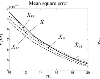
The estimation is performed for increasing number of measurementsm. As measure of the estimation quality, we use the empirical (relative) mean square error

eðmÞ ¼ 1

N XN

s¼1

kX0XX^ðsÞk2F

kX0kF2 ;

whereXX^ðsÞis the estimate computed for thes-th noise realization.

The ALS and the small sample modified ALS estimators are compared with the LS estimator

^ X

XlsvðATAÞ

y

ATCBTðBBT_Þy

;

and with the partial LS estimators, ^

X

XpavTLS solution of XB¼ ðA T_AÞy

ATC

and ^ X

XpbvTLS solution ofAX ¼CB

T_ðBBT_Þy_:

Figure 1 shows small sample size result for equally sized errors; the num-ber of measurements m is between 10 and 20. On the left plot is the mean square error of estimationeðmÞ for LS (dotted line), ALS (solid line), small sample modified ALS (dashed-dotted line) and partial LS (dashed lines) esti-mators. The plots are averaged forN¼200 noise realizations.

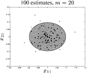
The right plot of Figure 1 illustrates application of the asymptotic normality results for confidence region computation, see Subsection 6.4. The

confidence region of xx^mvvecðXX^mÞ with 1a confidence probability is the

ellipsoid

E₁app_aðxx^mÞ ¼ xj ðxxx^mÞðS app_Þ1

ðxxx^mÞa

1 mðw

2 lÞa

;

whereðw_l2Þ_ais theaquantile of thew2_l distribution, i.e.Pðw_l2bðw_l2Þ_aÞ ¼a, and lis the number of degrees of freedom. Forxx^m in the example,l¼4.

In order to be able to visualize the results, we use the first two elements of ^

x

xm, denoted byxx^mð1:2Þ. Forxx^mð1:2Þ,l¼2 and the approximate asymptotic

covariance matrix is the upper left, 2 by 2 submatrix ofSapp.

The computed confidence regionE₀app_:9 ð^xxmÞform¼20 is shown as shaded

area on the plot. The symbol ‘‘₄’’ indicates the true value point½1 0T and the symbol ‘‘=’’ indicates the point estimatexx^Mð1:2Þ.

Figure 2 shows analogous results for equally sized errors for larger sample size;mbetween 20 and 100.

Figure 3, shows how the estimates are clustered. Again ‘‘4’’ corresponds to

the true value½1 0T. The ‘‘=’’ symbols correspond to 100 estimatesxx^Mð1:2Þ.

The shaded area is the ellipsoid,

E1aðxx^mÞ ¼ xj ðxxx^mÞS

1_ðxxx^ mÞa

1 mðw

2 lÞa

;

Fig. 2. Equally sized errors, result formAf20;. . .;100g

Table 1.Percentage of estimates inside inside

^

x

xMð1:2ÞAE0:9ðxx^Mð1:2ÞÞ 89%

^

x

xMAE0:9ðxx^MÞ 91%

described by the true asymptotic covariance matrixS, see (39), and centered at the true valuexx^mð1:2Þ.

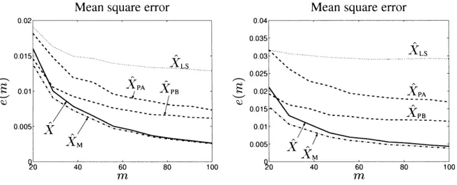
Figure 4 show the mean square error of the compared estimators for di¤erently sized uncorrelated errors (left plot) and for correlated errors (right plot).

9 Conclusion

We considered the multivariable modelAXB¼C. In the situation when the TLS estimator is inconsistent, we construct the ALS estimator, which is con-sistent. We gave the conditions of weak and strong consistency, and of asymp-totic normality. It turns out that the asympasymp-totic covariance matrix of the esti-mator does not depend upon the covariance structure ofCC. We introduced a~ small sample modification of the estimator, which has better properties for small samples and preserves the asymptotic properties of the estimator.

An open question is what are the optimality properties of the ALS estimator. In [KM00] for the modelAX ¼B in the scalar case it was shown that the ALS estimator is asymptotically e‰cient in the situation where V_AA~

is known exactly and Ebb~2_kl are known up to a constant factor. It would be interesting to check the following conjecture:

In the modelAXB¼Cthe ALS estimator is asymptotically e‰cient in the situation whereV_AA~and V_BB~ are known exactly and E~cc_il2 are known

up to a constant factor.

10 Appendix

10.1 Proof of (14)

We have

V_A01UA¼InþVA01ðAA~TAA~V_AA~Þ þV_A01ðAA~TA0þAT0AAÞ~: ð46Þ

Next

EkV1

A0 ðAA~TAA~V_AA~Þk2_FakV_A01k2EkAA~TAA~V_AA~k_F2 ð47Þ

andkV1 A0 k ¼l

1

minðVA₀Þ. By (ii) and (iii), we have

EkAA~TAA~V_AA~k2_F ¼

Xn

i;k¼1

var X

m

j¼1

~ a aji~aajk

!

¼ X

n

i;k¼1

Xm

j¼1

varð~aajiaa~jkÞaconstm;

thus by (iv)

EkVA01ðAA~TAA~V_AA~Þk2_Fa

constm

l2_minðVA0Þ

!0 asm!y; ð48Þ

this proves thatV1

A0 ðAA~TAA~V_AA~Þ ! p

0. Next

EkV1

A0 ðAA~TA0þAT0AAÞk~ 2 Fa

2

l2_minðVA0Þ EkAT

0AAk~ 2

F ð49Þ

and

EkAT0AAk~ 2 F ¼

Xn

i;k¼1

E X

m

j¼1

a_ji0aa~jk

!2

¼ X

n

i;k¼1

Xm

j¼1

ðaji0Þ 2

varðaa~jkÞ

aconstX

n

i¼1

Xm

j¼1

ða0 jiÞ

2

aconstlmaxðVA0Þ

and from (49) under assumption (iv) we have

V_A01ðAA~TA0þAT0AAÞ !~ p

0: ð50Þ

Now, (46), (48) and (50) imply the first relation in (14), and the second one in (14) holds similarly.

10.2 Proof of (15)

V_A01ðAT_A

0Þ ¼InþVA01AA~TA0;

and this converges in probability toIn, see Subsection 10.1. The second

10.3 Proof of (16)

We have

kV_A01ATCCB~ TV_B01k_Fa 1

lminðVA0ÞlminðVB0Þ

kATCCB~ Tk_F; ð51Þ

and

EkAT_CCB~ T_k2 F ¼

Xn

j¼1

Xp

k¼1

E X

m

i¼1

Xq

l¼1

aijcc~ilbkl

!2

¼ X

i;j;k;l

Ea2_ijvarð~ccilÞEb2kl

aconst X

m

i¼1

Xn

j¼1 Ea_ij2

! Xp

k¼1

Xq

l¼1 Eb2_kl

!

aconst ðlmaxðVA0Þ þmÞðlmaxðVB0Þ þqÞ:

Then from (51) we have

EkV_A01ATCCB~ TV_B01k2_FaconstðlmaxðVA0Þ þmÞ

l2_minðVA0Þ

ðlmaxðVB0Þ þqÞ

l2_minðVB0Þ ;

and this tends to zero, asm!y_,q!y_{by assumption (iv).}

10.4 Proof of Theorem 2

We have to show that in (14) to (16) the convergence is with probability one. After that the statement of Theorem 2 will follow from equation (13) for the estimatorXX.^

We use Lemma 1. First, see (46). Consider

EkAA~TAA~V_AA~k_Fr ¼E

Xm

i¼1

ð~aa_iTaa~iEaa~iT~aaiÞ

r

F

aconstmr=2;

because by (v)Ek~aak2raconst. Then

EkV_A01ðAA~TAA~V_AA~Þk_Fraconst

mr=2

lr_minðVA0Þ ;

Xy

m¼m0

mr=2

lr_minðVA0Þ <y

and by Borel-Cantelli lemma

Next, consider

kAA~TA0þAT0AkA~ Fa2kAT0AAk~ F

and

EkAT₀AAk~ _F2r¼E X m

i¼1

a0T_i ~aai

2r

F

aconst X

m

i¼1

ka0_ik2 !r

aconstlr_maxðVA0Þ:

Therefore,

EkV1

A0 ðAA~TA0þAT0AAÞk~ 2r

aconstl

r maxðVA0Þ

l2r_minðVA0Þ ;

Xy

m¼m0

lr_maxðVA0Þ

l2r_minðVA0Þ ay;

and by Borel-Cantelli lemma

V_A01ðAA~TA0þAT0AAÞ !~ 0 a:s:; asm!y:

Thus, see (46),V_A01UA!In a.s., as m!y. Similarly, UBVB01!Ip a.s., as

q!y_.

Secondly, in (15) we also have convergence a.s., compare with the proof of Theorem 1.

Thirdly, consider

E½kATCCB~ Tk_F2rjAA~;BB ¼~ E X m

i¼1

Xq

l¼1

aT_i cc~ilblT

2r

F

jAA~;BB~ 2

4

3 5

aconst X

m

i¼1

Xq

l¼1 E½kaT

i ~ccilblTk

2r_jAA~;BB~

þ X

m

i¼1

Xq

l¼1

E½ka_iTcc~ilblTk 2

jAA~;BB~ !r!

:

Now, Xm

i¼1

Xq

l¼1

E½ka_iTcc~ilblTk 2r

jAA~;BB~ aconstX

m

i¼1

kaik2r

Xq

l¼1

kblk2r;

and

E X

m

i¼1

Xq

l¼1

E½kaTi ~ccilblTk 2r

jAA~;BB~ !

Next,

E X

m

i¼1

Xq

l¼1

E½ka_iT~ccilblTk 2

jAA~;BB~ !r

aconstE X m

i¼1

kaik2

!r

E X

q

l¼1

kblk2

!r

aconst ðlr_maxðVA0Þ þmrÞðlrmaxðVB0Þ þqrÞ

Therefore

EkATCCB~ Tk_F2raconst ðlr_maxðVA0Þ þmrÞðlmaxr ðVB0Þ þqrÞ;

and, see (46),

EkV_A01ATCCB~ TV_B01k2r_F aconstl

r

maxðVA0Þ þmr

l2r_minðVA0Þ

l_maxr ðVB0Þ þqr

l2r_minðVB0Þ ;

Xy

m¼m0

Xy

q¼q0

lr_maxðVA0Þ þmr

l2r_minðVA0Þ

lr_maxðVB0Þ þqr

l2r_minðVB0Þ

¼ X

y

m¼m0

lr_maxðVA0Þ þmr

l2r_minðVA0Þ

! Xy

q¼q0

lr_maxðVB0Þ þqr

l2r_minðVB0Þ

!

<y:

Then for eache>0,

PðkV1

A0 ATCCB~ TVB01k>eÞa

1

e2rEkV

1

A0 ATCCB~ TVB01k 2r

and by Borel-Cantelli lemma with probability one the event

Dmq¼ fkVA01ATCBC~ TVB01k>eg

happens only for finite number of indices m and q. Then almost surely there exists m1¼m1ðoÞ and q1¼q1ðoÞ, such that for all mbm1, qbq1,

kV1

A0 ATCCB~ TVB01kae.

This means thatV1

A0 ATCCB~ TVB01 !0 a.s., asm!y,q!y.

We proved that in (14) to (16) the convergence is with probability one and Theorem 2 is proved. r

10.5 Proof of Lemma 3

We have

TAWA¼

1 t f

T

tqCTCftq p1ffiffi_tftqTCTA 1_ffiffi

t

p _AT_{Cftq A}T_AV~

A A

" #

¼ 1ffiffi t

p C0ftq A0

T

1 ffiffi t

p C0ftq A0

þ

1 tftqTCC~

T_CCf~ tq 0 0 0 þ 1 t f T

tqðC0TCC~þCC~ T_C

0Þftq p1ffiffi_t ftqTðC0TAA~þCC~ T_A

0Þ 1_ffiffi

t

p _ðAA~TC0þAT0CÞC~ ftq AT0AA~þAA~ T_A

0þ ðAA~TAA~V_AA~Þ

2 4

3 5

vH1þH2þH3:

10.5.1 Behavior ofH1

We haveH1b0, andH1 ¼

" H0

11 H120

H₂₁0 H₂₂0 # ; 1 mH 0 22¼ 1 mA T

0A0!VAy>0; see assumptionðviiÞ:

10.5.2 Behavior ofH2

We haveH2¼

H₁₁00 0 0 0 , 1 mH 00 11¼ 1 mt Xm

i¼1

Xt

k¼1

~ ccik

Xt

l¼1

~ ccil¼

1 mt

X

1aiam 1akat

~ cc_ik2 þ 2

mt X

1aiam 1ak<lat

~

ccikcc~ilvSAþSB:

We have

1 4ES

2 B¼

1 m2_t2

X

1aiam 1ak<lat

Eð~cc2

ikÞEð~ccil2Þaconst

mt2

m2_t2!0 asm!y;q!y:

Next, by assumption (xv) and by the law of large numbers

SA!Ecc~112 a:s: asm!y;q!y

H2! Ecc~2

11 0

0 0 " #

a:s:

10.5.3 Behavior ofH3

We prove that 1 mH3!

p

0. We writeH3¼

H₁₁000 H₁₂000 H₂₁000 H₂₂000

,

a).

1

m2E

1 tf

T tqC

T 0CCf~tq

2

¼ 1

m2E

1 tf

T tqCC~

T_C 0ftq

2

¼ 1

m2_t2E

Xm

i¼1

Xt

k¼1

c0_ikX

t

l¼1

~ ccil

!2

¼ 1

m2_t2

Xm

i¼1

Xt

l¼1

E~cc₁₁2 X

t

k¼1

c_ik0 !2

aconst 1 m2

Xm

i¼1

Xt

l¼1

ðc0 ikÞ

2

aconst 1

m2lmaxðVA0Þlmax

Xt

i¼1

b_i0b0T_i !

aconst t

m!0;

becauset¼oðp3ffiffiffiffim_{Þ. ThusH}000

11 ! p

0. b).

1

m2E

1 ffiffi t

p AA~TC0ftq

2 ¼ 1

m2_tE

Xn

k¼1

Xm

i¼1

~ a aik

Xt

l¼1

c0_il !2

aconst 1 m2_t

Xn

k¼1

Xm

i¼1

Xt

l¼1

c_il0 !2

aconst 1 m2

Xm

i¼1

Xt

l¼1

ðc0 ilÞ

2

aconst t

c).

1

m2E

1 ffiffi t p AT₀CCf~tq

2 ¼ 1

m2_tE

Xn

k¼1

Xm

i¼1

a_ik0 X

t

l¼1

~ ccil

!2

¼ 1

m2_t

Xn

k¼1

Xt

l¼1

E~cc₁₁2 X

m

i¼1

a0_ik !2

aconst 1 m2

Xm

i¼1

Xn

k¼1

ða0 ikÞ

2

aconst t

m!0:

From b) and c) we haveH₁₂000!p 0,H₂₁000!p 0. d). It was shown above thatH000

22! p

0, see section 10.1. Finally,H3! p

0.

10.5.4 End of proof

Summarizing Subsection 10.5.3, we have 1

mH3

F ¼ ffiffiffiffi t m r

Opð1Þ:

We need to know the behavior of the other blocks ofH1.

1 mH 0 11 ¼ 1 mt Xm

i¼1

Xt

l¼1

c_il0 !2

a 1

m Xm

i¼1

Xt

l¼1

ðc0 ilÞ

2

aconstt:

1

mH

0

21¼

1 mpffiffitA

T

0C0ftq¼

1

mA

T 0A0

1 ffiffi t

p X0B0ftq;

1 mH 0 21 F

aconstpffiffit;

and 1 mH 0 12 F ¼ 1 mH 0 21 F

We consider the matrix

MAv

1

mðH1þH2Þ:

It is positive semidefinite and we look fore0>0 such thatMAbe0_t Inþ1 with

probability tending to one. We have

MA

e0

t Inþ1¼

1 mH

0

11þ m1H

00 11 e0 t ₁ mH 0 12 1 mH 0

21 m1H

0

22 e0

t In

" #

:

Now, formbm0

1

mH

0

22

e0

t Inb 1

2lminðVAyÞ

e0

t

Inb

1

2lminðVAyÞ e0

In

b1

4lminðVAyÞ; ife0a 1

4lminðVAyÞ:

We apply Silvester’s criterion to the matrixMAe0_t Inþ1. We have for

e0a

1

4lminðVAyÞ; ð52Þ

det MA

e0

t In

¼det 1

mH1

þ 1 mH 00 11 det 1 mH 0 22 e0

t In

þe0Oð1Þ:

ð53Þ

The last term comes from 1 mH

0

11det m1H

0

22 e0

t In

and from the product of components_m1H₂₁0 ,_m1H₁₂0 ande0_t In. In both cases we havete0_t Oð1Þ ¼e0Oð1Þ.

Now, 1

mH1b0, therefore (53) implies

det MA

e0

t Inþ1

b 1

mH

00

11det

1

mH

0

22

e0

t In

const1e0;

with some const1>0, and a.s. we have

lim inf

m!y q!y

det MA

e0

t Inþ1

bEcc~₁₁2 detðVAyÞ const1e0>0;

if

e0<

1 const1

Ecc~₁₁2 detðVAyÞ: ð54Þ

Therefore ife0satisfies (52) and (54) then

MA

e0

with probability tending to one, and

lminðMAÞb

e0

t ;

with probability tending to one. We have

lmin

1

mðTAWAÞ

blminðMAÞ

1

mH3

blminðMAÞ

ffiffiffiffi t m r

Opð1Þ;

and with probability tending to one we have

lminðTAWAÞb

e0

t

ffiffiffiffi t m r

Opð1Þ:

But with probability tending to one

e0

t

ffiffiffiffi t m r

Opð1Þ>0,

ffiffiffiffi m t3

r

e0>Opð1Þ;

and the last holds because by assumptionm

t3!y. ThusTA>WAwith

prob-ability tending to one. Lemma 3 is proved. r

Acknowledgements. We thank two anonymous reviewers for their suggestions and corrections.

A. Kukush is supported by a postdoctoral research fellowship of the Belgian o‰ce for Scien-tific, Technical and Cultural A¤airs, promoting Scientific and Technical Collaboration with Cen-tral and Eastern Europe.

S. Van Hu¤el is a full professor with the Katholieke Universiteit Leuven. I. Markovsky is a research assistant with the Katholieke Universiteit Leuven.

This paper presents research results of the Belgian Programme on Interuniversity Poles of Attraction (IUAP V-22), initiated by the Belgian State, Prime Minister’s O‰ce – Federal O‰ce for Scientific, Technical and Cultural A¤airs of the Concerted Research Action (GOA) projects of the Flemish Government MEFISTO-666 (Mathematical Engineering for Information and Com-munication Systems Technology), of the IDO/99/03 project (K.U. Leuven) ‘‘Predictive computer models for medical classification problems using patient data and expert knowledge’’, of the FWO projects G.0078.01, G.0200.00, and G0.0270.02.

The scientific responsibility is assumed by its authors.

References

[Bar00] Baran S (2000) A consistent estimator in general functional errors-in-variables models. Metrika 51(2):117–132

[CRS95] Carroll RJ, Ruppert D, Stefanski LA (1995) Measurement error in nonlinear models. Number 63 in Monographs on Statistics and Applied Probability. Chapman & Hall/ CRC

[CS98] Cheng C, Schneeweiss H (1998) Polynomial regression with errors in the variables. J. R. Statistical Society B (60):189–199

[CST00] Cheng C, Schneeweiss H, Thamerus M (2000) A small sample estimator for a polyno-mial regression with errors in the variables. J. R. Statistical Society (62):699–709 [Ful87] Fuller WA (1987) Measurement error models. New York: Wiley

[GV80] Golub GH, Van Loan CF (1980) An analysis of the total least squares problem. SIAM J. Numer. Anal. (17):883–893

[KM00] Kukush A, Maschke E-O (2000) The e‰ciency of adjusted least squares in the linear functional relationship. Discussion Paper 208, SFB 386, Ludwig-Maximilians-University of Munich

[KMV01] Kukush A, Markovsky I, Van Hu¤el S. Consistent fundamental matrix estimation in a quadratic measuremnt error model arising in motion analysis. Technical Report 01-64, Dept. EE, K.U. Leuven, 2001. Accepted for publication in Computational Statistics and Data Analysis, Special Issue of Matrix Computations and Statistics

[KZ96] Kukush A, Zwanzig S (1996) On inconsistency of the least squares estimator in non-linear functional error-in-variables models. Preprint N96-12, Institut fu¨r Mathemati-sche Stochastik, Universita¨t Hamburg

[MM98] Mu¨hlich M, Mester R (1998) The role of total least squares in motion analysis. In Burkhardt H (ed) Proc. European Conference on Computer Vision (ECCV’98), Springer Lecture Notes on Computer Science, pages 305–321. Springer-Verlag, June [Ros70] Rosenthal HP (1970) On the subspaces ofLp_{ðp>2Þspanned by sequences of}

inde-pendent random variables. Isr. J. Math. (8):273–303

[VV89] Van Hu¤el S, Vandewalle J (1989) Analysis and properties of the generalized total least squares problemAXABwhen some or all columns inAare subject to error. SIAM J. Matrix Anal. 10(3):294–315