Information Processing in the Interaural Time Difference Pathway of the Barn Owl

Information Processing in the Interaural Time Difference

Pathway of the Barn Owl

Thesis by

Gestur Bj¨orn Christianson

In Partial Fulfillment of the Requirements for the Degree of

Doctor of Philosophy

California Institute of Technology Pasadena, California

2006

c 2006

Acknowledgements

Thanks are due first and foremost to my advisor, Masakazu Konishi, without whom this work would never have been done. Also I must thank my collaborator, Jos´e Luis Pe˜na, who recorded all of the NL data shown in this work. All members of the Konishi lab with whom I have had the pleasure of working have contributed in some manner to my research; I would like to particularly thank Ben Arthur, Brian Fischer, Sharad Shanbhag, and Teresa Nick, as well as Roian Egnor for a key piece of advice I wish I had heeded sooner.

I would also like to thank my committee members, Ralph Adolphs, Gilles Laurent, Jerry Pine, Shinsuke Shimojo, and Erik Winfree. Invaluable technical assistance was provided throughout this work by Chris Malek and Gene Akutagawa, as well as all the staff of the Office of Laboratory Animal Resources.

Peter Dayan, Peter Latham, Jennifer Linden, Richard Lyon, Ofer Mazor, Markus Meister, Peter Narins, and Maneesh Sahani have all provided me with helpful discussions on this material.

Abstract

Contents

Acknowledgements iv

Abstract v

List of Figures ix

List of Tables xi

1 Introduction 1

1.1 Overview of sound localization . . . 2

1.2 Sound localization cues . . . 3

1.3 The barn owl . . . 5

1.4 Anatomy of the sound localization pathway . . . 7

1.5 Computation of the interaural time difference . . . 10

1.6 Role of the post-laminaris ITD pathway? . . . 16

2 Methods 18 2.1 Surgery . . . 18

2.2 Electrophysiology . . . 19

2.3 Acoustic stimulation . . . 20

2.4 Data collection . . . 20

2.5 Modeling . . . 21

3.1 Methods . . . 25

3.1.1 Data collection . . . 25

3.1.2 Analysis . . . 26

3.2 Results . . . 30

3.2.1 General properties . . . 30

3.2.2 Effect of ITD on STRF . . . 36

3.2.3 Separability . . . 38

3.2.4 Variability . . . 41

3.3 Discussion . . . 43

4 Relationship between Spectral and ITD Tuning 48 4.1 Methods . . . 50

4.1.1 Data collection . . . 50

4.1.2 Analysis . . . 51

4.2 Results . . . 52

4.2.1 Nucleus laminaris . . . 52

4.2.2 Model of nucleus laminaris response . . . 54

4.2.3 ICcc . . . 59

4.2.4 Envelope coding . . . 61

4.3 Discussion . . . 62

5 Tuning to Interaural Time Difference 66 5.1 Methods . . . 67

5.1.1 Analysis . . . 68

5.1.2 Modeling . . . 69

5.2 Results . . . 70

5.2.1 Evolution of tuning across stimulus repetitions . . . 70

5.2.3 Rectification of response . . . 76 5.2.4 Model of ICcc neurons . . . 77 5.3 Discussion . . . 81

6 Summary of Results 91

A The Weiner-Khinchin Theorem 93

B Running Cross-Correlation 96

List of Figures

1.1 Binaural cues . . . 4

1.2 Sound localization pathway . . . 8

1.3 Jeffress model . . . 11

1.4 Phase-locking . . . 12

1.5 “Phase ambiguity” for complex signals . . . 13

1.6 Frequency convergence for elimination of phase ambiguity . . . 15

2.1 Example ISIHs for NL neurons . . . 21

3.1 Latency estimation . . . 29

3.2 Examples of spike-triggered averages . . . 31

3.3 Spike-triggered covariance . . . 32

3.4 Quadrature pairs . . . 34

3.5 Comparison of latency in quadrature pairs . . . 35

3.6 Dependence of latency on frequency . . . 36

3.7 Bandwidth as a function of nucleus and center frequency . . . 37

3.8 Iso-intensity frequency tuning curve bandwidth . . . 38

3.9 STRFs are independent of ITD . . . 39

3.10 Separability . . . 40

3.11 Fractional energy of the singular values . . . 41

3.12 STRF component power in tuned and untuned regions . . . 42

3.14 Variability in NL and ICcc . . . 44

4.1 NL ITD response curve . . . 53

4.2 Reverse correlation and ITD tuning . . . 55

4.3 Sampling rate compensation . . . 56

4.4 Iso-intensity frequency tuning and ITD tuning . . . 57

4.5 NL model response . . . 58

4.6 Rectification in ICcc ITD tuning curves . . . 59

4.7 Unrectified ICcc tuning curves . . . 60

4.8 ITD tuning curves in the physiological range . . . 63

5.1 ITD response curves . . . 71

5.2 ITD response across trials . . . 72

5.3 ITD response across trials (population) . . . 73

5.4 Physiological-range ITD response across trials . . . 74

5.5 ITD response within a single trial . . . 75

5.6 Comparison of dynamic range . . . 76

5.7 Rectification in ICcc tuning curves . . . 77

5.8 Rectification indices . . . 78

5.9 Reverse correlation of model ICcc neuron . . . 79

5.10 SAC of model ICcc neuron . . . 81

5.11 Reverse correlation of model ICcc neuron for fixedτs . . . 82

5.12 Reverse correlation of model ICcc neuron for fixedτm . . . 83

5.13 Binaurally uncorrelated responses . . . 86

List of Tables

2.1 Spiking model parameters . . . 22

Chapter 1

Introduction

The task of the nervous system can be grossly summarized as a three-step process: to encode information about the environment; to make decisions based on that encoded information about future actions; and to implement those actions. The first of these tasks is the duty of the sensory system, and the challenges it faces are remarkable. The world around us is vast and ever changing. Even taking into account the inherent limitations of our sensory organs, we are bombarded by enormous amounts of information. The sensory systems of the nervous system must first take in this information and then somehow reduce it to a manageable level, by efficient coding, discarding of irrelevant information, or combinations of the above. To study a sensory system is thus to attempt to answer the question of what information about a stimulus is encoded, and how.

Before this question can be tackled, however, the researcher must first be able to describe and analyze the stimuli he plans to use. From this perspective, hearing is a modality that offers consider-able advantage. A sound is simply a time-dependent pressure waveform, and hence one-dimensional. Because of this low dimensionality, sounds can be characterized using the large body of mathemat-ical work that has been done on one-dimensional signal analysis, permitting simple mathematmathemat-ical descriptions of complex stimuli. The ability to describe and manipulate complex properties of the signal in turn allows us to easily explore the dependence of neural response on even high-order characteristics of the signal.

of how neurons might implement these computations, or indeed whether the models are followed, and to what degree, the existence of a clear theoretical framework is an invaluable tool for the design of experiments.

There are a number of perceptual tasks in which audition plays a role. This research deals with the problem of sound localization. In particular, we focus on the neural processing of the interaural time difference between its initial computation and its convergence with the interaural level difference. Before that discussion begins, it is first necessary to provide background detail on the general nature of sound localization, as well as previous research on the neural mechanisms for its solution within the barn owl, the model used by this study.

1.1

Overview of sound localization

Audition is not an inherently spatial sense. Even though the responses of the primary receptors for both vision and audition are functions of stimulus intensity, the photoreceptors of the eye are arrangedspatiotopically, in a two-dimensional map of space. Conversely, the hair cells of the ear are arrangedtonotopically, arrayed across the cochlea as a map of frequency of the stimulus (von Bekesy 1960; Ruggero et al. 1997). Despite the lack of an explicit representation of space in the initial encoding of auditory information, animals and humans alike are capable of identifying the spatial source of a sound. The ability of animals to extract the position of a single source from auditory information represents a computational challenge that is simultaneously complex and well defined. The only inputs to the calculation are the two one-dimensional pressure waveforms that correspond to the sound at each ear, and the results of the computation can be reported using a single physical movement, usually either an eye or head saccade, or a pointing motion. The computations underlying sound localization have been studied for over two centuries using behavioral and physiological methods (Venturi 1796; Rayleigh 1876; Rayleigh 1907).

and Fay 1995). Since it is an active system, information can be extracted by comparing the returned signal to the original signal. This means echolocation can make use of sophisticated cues such as the Doppler shift, where changes in the spectrum of the emitted pulse are caused by the relative velocities between animal and detected object (M¨uller and Schnitzler 1999). In addition, because the echolocating animal is the one that creates the sound, it can use a sound optimally suited to the environmental conditions (Schnitzler and Kalko 2001). Conversely, sound localization is a passive system, with no prior knowledge of or control over the sound to be localized. As a result, it is theoretically less precise than echolocation. From an ethological perspective, however, passive sound localization offers some advantages. Echolocation is energetically expensive (Speakman, Anderson and Racey 1989), while sound localization requires no additional energy expenditure during the search for prey. Additionally, prey can develop countermeasures to try to counteract echolocation (Greenfield and Baker 2003; Waters 2003), while there is no way to avoid passive sound localization other than the relatively unhelpful strategy of “don’t make noise.”

1.2

Sound localization cues

There are several cues present that can be used to determine the position of a sound (Blauert 1997). Primary among these are the binaural cues, arising from the differences in the sounds at the two ears (fig. 1.1), the use of which were first demonstrated by Rayleigh (1907).

The interaural level difference (ILD; sometimes used interchangeably with the interaural intensity difference, or IID, though the two terms are technically different) arises due to occlusion of the sound by the head at the far ear. For a sound source to the right of the animal, the head will cast an acoustic “shadow” over the left ear, reducing the sound intensity there (fig. 1.1). This effect is not uniform across frequencies. For low frequencies, diffraction causes the incoming waveform to propagate past the head with relatively little reduction in intensity (Shaw 1974). As a consequence, ILD cues are theoretically better suited to high-frequency signals.

Interaural Level Difference

Interaural Time Difference

Acoustic shadow Sound source

Paths to the two ears are of different lengths

Figure 1.1. An illustration of binaural cues for the purposes of sound localization.

it arrives at the left (fig. 1.1), resulting in an ongoing temporal disparity for that sound between the copies at the two ears. The maximum ITD an animal can perceive is limited by the size of the head, as the maximal difference in path lengths from sound source to ears is given by the interaural separation. In general, this maximum ITD is quite small, on the order of about 630 μs for the human (Blauert 1997) and 180μs for the owl (Moiseff and Konishi 1981). Thus, to use the ITD as a sound localization cue, the animal must be able to detect interaural disparities on a very short time scale. For reasons we will discuss in detail in section 1.5, this means that the computation of ITD is generally easier at low frequencies.

Yin 1998). However, the evidence is that motion-based cues from the movement of the head in humans (whose outer ears are fixed) contribute, at best, weakly to localization performance (Pollack and Rose 1967; Thurlow and Runge 1967).

In the majority of systems that have been studied, including all mammalian systems, the sym-metry of the placement of the ears on the head causes both the ITD and the ILD to encode position along the horizontal plane, with ITDs being used for low frequencies and ILDs being used for high frequencies. This interaction is referred to as the duplex theory. In humans, psychophysics confirms that monaural cues are used to determine elevation (Middlebrooks and Green 1991).

1.3

The barn owl

The barn owl (Tyto alba) is a nocturnal predator. Despite a well-developed visual system (Pettigrew and Konishi 1976; van de Willigen, Frost and Wagner 1998), light levels in the wild often fall below the levels at which the owl can see (Dice 1945; Curtis 1952), indicating that owls must use some non-visual sense to hunt. It was hypothesized that owls might have vision extending into the infra-red spectrum (Vanderplank 1994), though this was rapidly disproven (Matthews and Matthews 1939; Hecht and Pirenne 1940). Dice (1945) noted that in darkness owls searching for prey would occasionally touch dead mice without apparently noticing it, arguing against a role for olfaction in hunting. Similarly, Curtis (1952) found a direct correlation between light intensity and the ability of an owl to navigate barriers in its flight path, which made it unlikely that the source of the owl’s hunting ability lay in either echolocation or the ability to perceive infra-red radiation.

Motivated by these reports, researchers began to explore the neural mechanisms that underlie the barn owl’s localization ability. It was found that the position of sounds are represented in an explicit, spatially organized map in the external nucleus of the inferior colliculus (ICx) within the owl’s midbrain (Knudsen and Konishi 1978a, 1978b), providing a direct correlate between behavioral reports and neurophysiological responses. While the superior colliculus of cat (Middlebrooks and Knudsen 1984), ferret (King and Hutchings 1987), and guinea pig (Sterbing, Hartung and Hoffmann 2002) have been reported to have maps of auditory space in register with a visual map of space, it is only in the barn owl that an exclusively auditory map of space, such as that seen in ICx, has been reported. This map, unconfounded by visual cues and providing a neural correlate to the localization behaviors, makes the owl an excellent model for the study of the mechanisms of sound localization. There are several crucial differences between the localization mechanisms of the barn owl and mammalian species, including the human. The range of frequencies that the owl can perceive extends only up to about 12 kHz (Konishi 1973), while the hearing range of humans extends to about 20 kHz. Within this range, the owl can localize well using frequencies from 1 to 8 kHz, and preferentially uses frequencies in the comparatively narrow range of 4 to 8 kHz (Knudsen and Konishi 1979); conversely, mammals appear to use the entirety of their range for localization. In the barn owl, an asymmetry in the owl’s outer ears (Norberg 1977) results in ILD coding for elevation (Knudsen and Konishi 1979), while monaural cues are not used (Egnor 2000); the preference for high frequencies ensures that diffraction of the sound about the head does not have a major influence on the use of the ILD cue. As a consequence of ILD coding for elevation, the owl must use ITD to encode azimuth throughout its sensitive frequency range (Knudsen and Konishi 1979), while most other animals only rely on ITD for frequencies less than 2 kHz.

of the neurons of the midbrain and the behavioral capabilities. In addition, the use of the two binaural cues to resolve orthogonal directions, the lack of use of the monaural cues, and the absence of mobile pinnae greatly reduces the number of variables to be considered in analyzing the system. With the understanding that comes from studying such a specialized system, it becomes easier to recognize optimizations and trade-offs that will be made by non-auditory specialist species.

1.4

Anatomy of the sound localization pathway

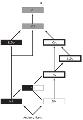
The organization of the neural structures that precede ICx with its spatial map have been studied extensively. A primary result of this exploration was the discovery of parallel pathways for the processing of ITD and ILD (fig. 1.2; Sullivan and Konishi 1984; Takahashi and Konishi 1988a, 1988b). As each auditory nerve fiber enters the brain, it bifurcates to terminate in both of the cochlear nuclei, nucleus magnocellularis (NM) and nucleus angularis (NA) (Carr and Boudreau 1991). Neurons of nucleus magnocellularis encode the phase of tonal stimuli for frequencies up to 9 kHz, and have reduced variation in firing rate as a function of stimulus intensity compared to the auditory nerve fibres (Sullivan and Konishi 1984; K¨oppl 1997b). Conversely, neurons of nucleus angularis do not phase-lock, and their dynamic ranges in response to changes in stimulus intensity are very large (Sullivan and Konishi 1984). Thus, the two nuclei are specialized to process phase or time information and intensity information, respectively.

NA projects contralaterally to the nucleus dorsal lemnisci lateralis pars posterior (LLDp; previ-ously known as the nucleus ventralis lemnisci lateralis pars posterior, VLVp; Takahashi and Konishi 1988a). This projection is excitatory, and combined with an inhibitory input from the contralateral LLDp (Takahashi and Keller 1992) produces a sigmoidal tuning to ILD in LLDp, with a preference for contralaterally-dominated ILDs (Moiseff and Konishi 1983; Manley, K¨oppl and Konishi 1988). NA also has projections to the superior olive (SO; Takahashi and Konishi 1988a), the nucleus ventral lemnisci lateralis (LLv, not shown on fig. 1.2; Takahashi and Konishi 1988a), and the lateral shell of the central nucleus of the inferior colliculus (ICcl; Takahashi and Konishi 1988b).

Auditory Nerve

NA NM

NL

LLDa ICcc

ICcl ICx

LLDp

SOO

Figure 1.2. A simplified schematic of the sound localization pathway. The ILD pathway is shown in black, the ITD pathway in white, and the sites in which the cues converge are grey. The nuclei of the closed loop that is the focus of this thesis are emphasized with the heavy black border.

nucleus of the inferior colliculus (ICcc; Takahashi and Konishi 1988b).

SO receives excitatory projections from NA and NL (Takahashi and Konishi 1988b; Lachica, R¨ubsamen and Rubel 1994). The neurons of SO do not encode phase, and are relatively insensitive to binaural cues (Moiseff and Konishi 1983). GABAergic projections from SO to NL and to NM (Lachica, R¨ubsamen and Rubel 1994) have led to the hypothesis that SO serves to eliminate the effect of stimulus intensity on the tuning of NL neurons (Lachica, R¨ubsamen and Rubel 1994; Pe˜na et al.1996; Dasika et al.2005).

Following NL in the ITD pathway, LLDa in turn projects to ICcc (Moiseff and Konishi 1983) and to the nucleus basalis (Wild, Kubke and Carr 2001), which is outside our consideration. There are no reports that LLDa receives inputs other than from NL. ICcc then projects to the ICcl (Takahashi, Wagner and Konishi 1989), as well as to nucleus ovoidalis in the thalamus (Proctor and Konishi 1997; Cohen, Miller and Knudsen 1998). Both LLDa (Moiseff and Konishi 1983; Albeck and Konishi 1995) and ICcc (Wagner, Takashi and Konishi 1987, 2002) are tuned to ITD, with a lack of sensitivity to intensity or ILD on a par with the neurons of NL, and their ITD responses are still ambiguous.

There is a second continuation of the localization pathway other than the tectal one described above, commonly referred to as the forebrain pathway. Both ICcl and ICcc project to NO, while ICx does not (Knudsen and Knudsen 1983; Proctor and Konishi 1997; Cohen, Miller and Knudsen 1998; Arthur 2005). From NO, there is a projection through Field L to the arcopallium (previously called archistriatum; Cohen, Miller and Knudsen 1998), where space-specific neurons can also be found (Cohen and Knudsen 1995). While the space-specific neurons of arcopallium do not have a spatiotopic map, microstimulation in either arcopallium or OT will result in head saccades (du Lac and Knudsen 1990; Masino and Knudsen 1990; Knudsen, Cohen and Masino 1995).

In this research, our interest lies in issues relating to the computation of ITD. As such, the nuclei of interest are those highlighted in figure 1.2. While the mammalian sound localization pathway lacks the clear segregation of that of the barn owl, and there is yet to be identified any equivalents to ICcl or the forebrain or tectal pathway, mammalian homologues for NM (the anteroventral cochlear nucleus, or AVCN), NL (the medial superior olive, or MSO), and ICcc (the central nucleus of the inferior colliculus, or ICc1), as well as a more tentative homology for LLDa (the dorsal nucleus of the lateral lemniscus, or DNLL) have been identified.

1.5

Computation of the interaural time difference

Jeffress (1948) was the first to formulate the coincidence detection model for the computation of ITDs. In the Jeffress model, a series of neurons are connected bilaterally to the two ears with calibrated delay lines. The input spikes to these neurons encode timing properties of the auditory stimulus, and the neurons fire only when they receive coincident inputs from both sides. In this arrangement, the only coincidence detector that will fire is the one where the difference in propagation times for the delay lines from either side precisely balances the ITD, resulting in a place code of ITD (fig. 1.3). Thus, there are three requirements that must be met for the auditory system to implement the Jeffress model: there must be encoding of the ongoing time (or, equivalently, phase)

Sound source

Acoustic delay

Coincidence detectors Neural

delay

Difference in acoustic delays = 0

Difference in neural delays = 0

Difference in

acoustic delays = _+x

Difference in

neural delays = _–x

Figure 1.3. A schematic of the Jeffress model. Coincidence detectors are connected by a series of delay lines to the two ears; the delay lines are arranged such that the difference in the neural delays from either ear varies across the family of coincidence detectors. When the sound source is equidistant from the two ears, then only the coincidence detector whose neural delay lines are of the same length will receive inputs at the same time, and hence be active (left). When the sound source moves, so that there is an ITD of +x, only the coincidence detector whose neural delay lines have the same absolute difference but reversed in sign will receive coincident input (right).

of the stimulus, there must be neurons that can operate as coincidence detectors, and the inputs to the coincidence detecting neurons from the two sides must be delayed with respect to each other in a manner that is systematic across the neuronal population.

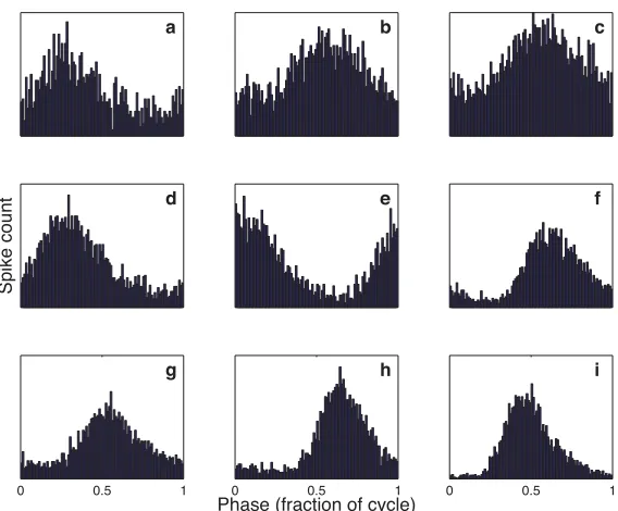
Recordings in the auditory nerve and NM reveal a tendency of these neurons, when stimulated with a tone, to fire preferentially for a particular phase of the input signal (fig. 1.4; Sullivan and Konishi 1984, K¨oppl 1997b). This provides in a straightforward manner an encoding of the ongoing time of the tone: each spike signals the reoccurrence of the preferred phase.

d

Spike count

a b c

e f

0 0.5 1 g

0 0.5 1 h

Phase (fraction of cycle)

0 0.5 1 i

Figure 1.4. Examples of phase-locking in the auditory nerve of the barn owl. Each fiber was stimulated with a tone of its preferred frequency. Spike times were converted to phase relative to the stimulus, and then a histogram of these phases was plotted. Note that while a peak in the phase histogram is apparent in all cases, it is also true that spikes occur at all phases, with this being more pronounced for higher-frequency neurons (a: unit 650.01, 7,500 Hz; b: unit 650.02, 7,750 Hz; c: unit 650.03, 7,500 Hz;d: unit 650.08, 5,750 Hz;e: unit 650.12, 5,500 Hz;f: unit 650.14, 4,750 Hz; g: unit 650.18, 4,500 Hz;h: unit 650.19, 3,500 Hz;i: unit 650.20, 2,250 Hz).

detecting time differences of frequencies below 1 kHz push the limits of what can be done with neural hardware, and it is for this reason that most animals use ITDs only for low-frequency signals. The owl can phase-lock over an enormous frequency range, at frequencies up to 9 kHz (K¨oppl 1997b). At the same time, there is still a decline in the quality of phase-locking with increasing frequency (fig. 1.4).

to ongoing time encoding of stimuli regardless of the spectral properties of the stimuli. This is partly convention, but is validated by the bandpass properties of the cochlea. Neurons throughout the ITD pathway, and the auditory nerve and NM in particular, are responsive to only a very narrow range of frequencies. Even white noise is thus effectively narrowband noise from the perspective of a single unit, and narrowband noise shares many of the features of tones. In particular, periodic stimuli such as tones are phase ambiguous: that is, without reference to an absolute end-point, it is impossible to distinguish between any given periodic signal and that same signal shifted in time by integer multiples of the period. Narrowband noise is not periodic; however, for small time displacements, it can be ambiguous in a manner similar to that seen in tones (fig. 1.5).

Broadband

a

Band−passed

b

Figure 1.5. a: A 1 ms segment of broadband noise (1–10 kHz) is plotted (solid line), and then shifted by 200μs and plotted again (dashed line). Note that at any given time, the curves have very little relationship to each other. b: The noise segment as used inahas been band-passed to have a 1 kHz bandwidth centered on 5 kHz, and plotted as before. The shift of 200μs corresponds to the period of the center of the band-pass filter. It can be seen that there is a great deal of correspondence between the time-shifted versions now, though this correspondence will fall off as larger time shifts are used.

Finally, Carr and Konishi (1990) observed phase-locking in NL neurons. If NL neurons are coincidence detectors, this is expected: the output spikes of NL will be directly related to the timing of its phase-locked inputs, and hence will be phase-locked themselves. NL neurons are driven by monaural stimulation as well as binaural stimulation, and the monaural response is also phase-locked. The preferred phase in monaural stimulation is given by the modulus of the conduction delay by the period of the stimulating frequency. Thus, the difference in preferred phase between ipsilateral and contralateral stimulation is equal to the true difference in conduction delays (called the characteristic delay, or CD) up to some integer multiple of the period of the frequency. So therefore, in a coincidence detector, presenting tones with an ITD that is equal to the difference in monaural phases but reversed in sign should elicit a maximal response; using an ITD that corresponds to a 180◦ shift in phase should result in a minimal response. This turns out to be the case (Carr and Konishi 1990), confirming that NL neurons act as coincidence detectors. Thus, all elements are present, and the Jeffress model stands as the description for how ITD is computed in the barn owl’s auditory pathway.

Figure 1.6. For a family of phase-ambiguous signals of different frequencies (dashed lines) but with one peak (the CD) in register, the side peaks will be out of phase with respect to each other (illustrated with thethin solid lines). The sum of these curves (heavy solid line) will have a maximal peak at the time of the CD alone.

The basic mechanism by which this ambiguity is resolved is frequency convergence (Mazer 1998; Saberi et al.1999). A phase-ambiguous neuron stimulated with broadband will have a peak response at its CD, and at ITDs that correspond to the CD plus some integer multiple of the period of the center frequency of its associated band-pass filter (fig. 1.5). A neuron of the same CD but different preferred frequency will thus have its secondary peaks at different ITDs. By summing across a population of such neurons with different preferred frequencies, it is possible to reinforce the peak at CD while the side-peaks will destructively interfere with each other, resulting in a single unambiguous peak. In the barn owl, the process of frequency convergence has been shown to begin in ICcl (Wagner, Takashi and Konishi 1987; Mazer 1995, 1998).

has not been unequivocally demonstrated (Smith, Joris and Yin 1993; Beckius, Batra and Oliver 1999). Related to this, McAlpine, Jiang and Palmer (2001) reported that in the guinea pig, CDs consistently fell outside the physiological range of ITDs as estimated by the interaural separation, though this work was done in ICc, and not MSO; Sterbing, Hartung and Hoffmann (2003) have argued that the observed CDs fall within the range predicted by the head-related transfer functions, as low frequency sounds distort about the head and pinnae, creating a longer path length. However, from the perspective of the computation of ITD, this is not a critical point: the distribution of CDs is of importance in the problem of decoding position from a range of ITD responses across a neuronal population (Harper and McAlpine 2004), and not an issue of how those ITD responses develop. Similarly, because mammals generally use ITD cues for sound localization only at frequencies below 2 kHz, phase ambiguity does not present a serious complication.

1.6

Role of the post-laminaris ITD pathway?

In the previous section, we described how the ITD was computed in NL, and how the problem of phase ambiguity was resolved in ICcl. However, this raises an interesting question. Between NL and ICcl lie the nuclei LLDa and ICcc (fig. 1.2). Both are exclusively tuned to ITD. In fact, the published data on their response properties suggests that their tuning is similar to that of NL (Moiseff and Konishi 1983; Wagner, Takashi and Konishi 1987; Albeck and Konishi 1995; Wagner, Mazer and von Campenhausen 2002). Since frequency convergence does not occur until ICcl (Wagner, Takashi and Konishi 1987; Mazer 1995, 1998), what role does the post-laminaris ITD pathway fill?

The simplest explanation is that it serves as a relay station, but we may dismiss this out of hand. This is not a single nucleus, but two; if the purpose was a relay, then presumably the NL– ICcc projection alone would suffice. In addition to this, ICcc and ICcl are subdivisions of the same nucleus, so that a direct projection from NL to the ICcl would be at best marginally longer, making it unlikely that a relay is required.

in response properties is regularly exploited to use ICc as a substitute for recording in MSO (for an example, see Yin, Chan and Carney 1987).

Chapter 2

Methods

Methods limited to a particular experiment will be described in the appropriate chapter.

2.1

Surgery

The protocol for this study followed the NIH Guide for the Care and Use of Laboratory Animals and was approved by the Institutes Animal Care and Use Committee.

sessions. The craniotomy was packed with gelfoam and sealed with dental cement, and the scalp was sutured closed. Following the surgery, analgesics (ketoprofen, 10 mg/kg, Ketofen, Merial) and antibiotics (oxytetracycline, 4 mg/kg, Maxim-200, Phoenix Pharmaceutical) were administered. The owl was kept in a heated cage until it recovered, at which point it was returned to the home cage. Weight was monitored from recording session to recording session, and the owl was given at least a week’s rest between sessions.

2.2

Electrophysiology

Single neurons of NL were isolated and maintained by a loose patch method in which a glass patch electrode served as a suction electrode, allowing us to hold neurons for a long time. Electrodes were prepared from 1.0 mm borosilicate glass (World Precision Instruments) using a micropipette puller (Sutter Instruments P-87). Electrodes were filled with a patch solution (in mM: K-gluconate 100, EGTA 10, HEPES 40, MgCl₂ 5, Na-ATP 2.2, Na-GTP 0.3), and impedance varied from 4 to 10 MΩ. Neural signals were serially amplified by an Axoclamp-2A (Axon Instruments) in the conventional current-clamp bridge mode, and further amplified and filtered with a custom-made device (B.E.S.μM-200). NL neurons were identified stereotaxically and by their response properties: in the owl’s brainstem, only NM and NL produce neurophonics, and of these, only NL has ITD tuning.

In both cases, a spike discriminator (SD1, Tucker Davis) converted neural impulses into TTL pulses for an event timer (ET1, Tucker Davis), which recorded the timing of the pulses. A computer running a custom software program (XDPHYS, written by J. A. Mazer, and modified by B. J. Arthur and C. Malek; available for download at ftp://ftp.etho.caltech.edu/pub/xdphys) was used for stimulus synthesis and online data analysis.

All recordings were done in a double-walled soundproof chamber (Industrial Acoustics Company, Inc.).

2.3

Acoustic stimulation

An earphone assembly consisting of a Knowles ED-1914 speaker, a Knowles BF-1743 damping device, and a Knowles EA-1939 microphone delivered sound stimuli. These components are encased in an aluminum cylinder that fits into the owl’s ear canal. The gaps between the cylinder and the ear canal were filled with silicon impression material (Gold Velvet II, All American Laboratories). At the beginning of each experimental session, the earphone assemblies were automatically calibrated. The computer was programmed to equalize sound pressure level and phase for all frequencies within the frequency range relevant to the experiment (500–13,000 Hz).

Tonal and broadband stimuli 100 ms in duration and sampled at 48,077 Hz were presented at a rate of approximately twice per second. Broadband stimuli were bandpassed to contain signal only from 500–12,000 Hz or from 1,000–12,000 Hz, depending on the preferred frequency range of the unit under study. Signals were gated at rise and fall with a 5 ms linear ramp to prevent onset effects. We used PA4 digital attenuators (Tucker Davis) to vary stimulus sound levels.

2.4

Data collection

that elicited the maximal response; when possible, the estimate was confirmed afterwards using a family of tonal ITD tuning curves.

Iso-intensity frequency tuning curves were obtained for sound levels 20 to 30 dB above threshold with randomized sequences of stimulus frequencies in steps of 100 Hz at the CD of the neuron. Frequency tuning curves were characterized by their width (W₅₀), center frequency (F₅₀) and best frequency (BF). W50 is the range of frequencies over which the cells discharge rate was equal to 50% of the difference between the maximal discharge rate and the spontaneous level. The frequency at the center of W₅₀ was defined as F₅₀. BF is defined as the frequency that elicits the maximal discharge rate in an iso-intensity frequency-tuning curve.

In a single neuron, the sound intensities used for all protocols were the same.

2.5

Modeling

The spiking models in this paper are inhomegenous Poisson processes that follow the implementation given in Zhang et al.(2001). However, for NL and ICcc, we used a different choice of history function. NL neurons have a characteristic inter-spike interval histogram (fig. 2.1) which is not well matched by a sum of exponentials. Instead, a history function based on a hyperbolic tangent was used:

H(t) =

⎧ ⎪ ⎪ ⎨ ⎪ ⎪ ⎩ −1

c3tanh(π

t−t₁−R_A−c₀

c1 +c2) (t−t1)≥RA

1.0 (t−t₁)< RA

whereRAis the absolute refractory period,t₁is the time of the last spike, and thecxare parameters.

0 5 10 0

100 200

a

0 5 10 0

100 200 300 _b

Inter−spike interval (ms)0 5 10 0

50 100 c

0 5 10 0

50 100 150

# of spikes

d

For NM, a sum of exponentials was used:

H(t) =

⎧ ⎪ ⎪ ⎨ ⎪ ⎪ ⎩

c0eRA−c(1t−t1 ) _+c2eRA

−(t−t1)

c3 _(t−_t1)≥_RA

1.0 (t−t1)< RA

though strictly speaking,c₂ was set to zero, and thus a single exponential was used.

The parameter values were chosen by hand to provide a reasonable approximation to the ap-propriate ISIH, though an inhomegenous Poisson process is incapable of accurately reproducing the ISIHs of NL. The values of the parameters used are given in table 2.1.

Table 2.1. Parameters used in the inhomogenous Poisson process

NM NL ICcc

RA 0.6 ms 1 ms 1 ms c₀ 1.0 0.003 0.0015 c₁ 0.2 0.003 0.0015

c₂ 0 1 1

Chapter 3

Spectrotemporal Receptive Fields

There is considerable evidence that the time-dependent structure of auditory signals is a major factor in the task of sound recognition. Fine temporal structure is a significant determinant in the discrimination and recognition of bird song (Brenowitz 1983), for example, and evidence suggests that intact temporal information permits the comprehension of speech even with degraded spectral cues (Drullman, Festen and Plomp 1994; Shannon et al. 1995; Wright et al. 1997). To process this information, the animal requires an encoding of the spectral properties of the stimulus as a function of time. When considered at the level of a single neuron, the combinations of frequencies and temporal profiles to which the neuron is responsive is referred to as thespectrotemporal receptive

field (STRF).

open as to which of these nuclei lead to the STRFs of ICcl, or if a combination of both is required. However, the initial nuclei of the ITD pathway, the auditory nerve (K¨oppl 1997b), NM (K¨oppl 1997b), and NL (Carr and Konishi 1990; Pe˜na et al. 1996) phase-lock when presented with tonal stimuli: they fire preferentially at a particular phase of the stimulating frequency. This link between a property of the stimulus and spike timing in the case of tonal stimuli suggests that there might be significant spectrotemporal tuning in the case of complex stimuli. Indeed, a link between phase-locking and spectrotemporal tuning for complex stimuli has been demonstrated in the auditory nerve of mammals (de Boer and de Jongh 1978; Eggermont 1993; Kim and Young 1994; Lewis, Henry and Yamada 2002; Louage, van der Heijden and Joris 2004). Thus, the ITD pathway is a reasonable candidate for the source of spectrotemporal tuning in ICcl.

In addressing a possible role of ICcc in the context of the post-laminaris pathway, its spectrotem-poral tuning is a logical place to commence. Unlike the auditory nerve, NM, and NL, ICcc does not phase-lock to tonal stimuli. At the same time, the temporal resolution required to produce phase-locking at the frequencies of interest in the barn owl is on the order of tens of microseconds (K¨oppl 1997b). It is entirely reasonable to believe that such high-quality temporal resolution can be degraded and still provide information about the instantaneous spectral properties of a stimulus with temporal resolution of use to the organism. In partial support of this hypothesis is the fact that ICcc projects directly to the auditory thalamus, which in turn projects to Field L, the avian homologue to the auditory cortex of mammals (Proctor and Konishi 1997; Cohen, Miller and Knud-sen 1998). Conversely, it might be that there is no stimulus-locking preKnud-sent in any form in ICcc; this would mean that the firing rate of an ICcc neuron is a function solely of ITD, which would simplify the task of extracting the position of the sound source.

to nucleus laminaris. Our results demonstrate that the STRFs of neurons throughout this ascending pathway are similar, despite the loss of phase information in the transition from NL to ICcc. This suggests that phase is of relevance primarily for the computation of ITD, and is encoded in the output of NL as an artifact of the computation of ITD, but also that high temporal resolution information about the envelope of the stimulus is preserved throughout the ITD pathway.

3.1

Methods

See chapter 2 for general methods.

3.1.1

Data collection

The occurrence of a spike is assumed to be related to the occurrence of a stimulus feature to which the neuron is sensitive. To determine the stimulus features to which the neuron is sensitive we used reverse correlation (de Boer and de Jongh 1978). In this method, we first compute the pre-event

stimulus ensemble (PESE): a matrix in which row n contains the segment of the stimulus that

preceded spiken. By examining the statistical properties of this matrix it is possible to determine the stimulus features that precede, and presumably elicit, spikes.

Data for reverse correlation were obtained by presenting 100 ms broadband signals at the best estimate of the characteristic delay of each neuron until a large number of stimulus-evoked spikes (NM: 7,330 ±4,250; NL: 2,909 ±1,343; ICcc: 2,792 ±1,352) that occurred between 40 ms after stimulus onset and the end of the stimulus were collected. Onset transients in the neural response of these nuclei are generally gone within 20 ms of stimulus onset. The time window of the reverse correlation (e.g., the amount of stimulus preceding each spike that was considered in the analysis) was 20 ms. Hence, the first 40 ms of response was removed to prevent the onset transient from appearing within the stimulus window. For each stimulus presentation, the signal was synthesized

de novo to avoid correlation artifacts, and stimuli using a second ITD (or intensity, in the case of

NM) were interleaved during the collection to prevent any effects of habituation to ITD.

protocol as reverse correlation, except that the stimuli were repeated presentations of the same broadband stimulus.

3.1.2

Analysis

Principal components analysis (PCA) of anm×m matrixM produces eigenvaluesλi, i= 1. . . m and a matrix of eigenvectors X such thatM =XΛX−1, where Λ(i, i) = λi and is zero elsewhere. The eigenvectors of M can be thought of as an optimal set of orthogonal axes for describing the data, and the corresponding eigenvalues describe the relative importance of that dimension. Smaller eigenvalues indicate that the corresponding eigenvector contributes little to the overall variance of the data, and can, if sufficiently small, be neglected.

PCA requires that the original data matrix be square. The singular value decomposition (SVD) can be thought of a generalization of PCA which removes this restriction. An m×nmatrixM is represented byM =UΛVT, whereU ism×m, V isn×n, and Λ is anm×ndiagonal matrix whose entries are the singular values λi of M. The fractional energy of a singular value λi is given by λ2_i/_jλ2_j, and is a measure of the relative contribution of the associated singular vector pair to the reconstruction of the overall matrix. The fractional energy ofλ₁ is equal to 1−α_SVD, whereα_SVD is the degree of inseparability defined by Depireux et al.(2001). In this work, whenever we compute the SVD we first subtract off the mean of M; otherwise the first singular value is dominated by a constant component. Since we use PCA only for the analysis of the covariance matrix, which is guaranteed to have mean 0, this step is not required there.

To determine significant second-order spike-triggered effects, the covariance matrix of the PESE was computed. Covariance is a statistical measure which can be thought of as the two-dimensional equivalent of the variation. The covariance of two random variablesxandy is given by:

Cov(x, y) = E[xy]−E[x]E[y]

correspond to the values of the stimulus at a precedence oft. This gives a matrix C, whose (i, j)th element is given by:

C₍i,j) = Cov(PESEi,PESEj)

where PESEi is the random variable that describes the value of the stimulus at a precedencei. To analyze the covariance matrix, we used PCA. This gives a family of eigenvectors, and we would like to demonstrate that we can safely disregard the majority of them. Fractional energy is an insufficient standard to make this argument except in the case of extreme values, as it does not provide a criterion for significance. Instead, we proceed by constructing a first-order model. By design, such a first-order model does not have second-order effects (i.e., it will have no significant covariance eigenvectors). If the distribution of eigenvalues in the data is significantly different from the distribution seen in the first-order model, then we can conclude that there are significant second-order effects present in the data. The first-order model assumes firing rate is related to the convolution of the spike-triggered average and the stimulus. A nonlinear weighting function of firing rate as a function of filter output was recovered using the method of Rust et al.(2004): a histogram of the inner products of all pre-event stimuli and the spike-triggered average was computed, and then piecewise normalized by the histogram of the inner products of all possible stimuli segments within the presented stimulus set and the spike-triggered average. The resulting histogram thus gives the probability of spiking as a function of the inner product of the stimulus and the spike-triggered average, and was fit with an asymmetric parabola of the form:

f(x) =

⎧ ⎪ ⎪ ⎨ ⎪ ⎪ ⎩

a₁x2+b x≤0 a₂x2+b x >0

through gradient descent to match the model’s mean firing rate to the data (see section 2.5). The spiking model was used to generate 100 PESEs of the same size as the original data PESE, thus giving a family of eigenvalue distributions for their respective covariance matrices. An eigenvalue of the data covariance was considered significant if it and all eigenvalues greater in magnitude differed from the model distribution by at least two standard deviations.

Power spectral density (PSD) was estimated with the MATLAB implementation of Thomson’s multi-taper method with the time-bandwidth product set to 5/2. We use three characterizations of the spectral properties of a signal. BW₁₀ is the 10 dB bandwidth of the signal; that is, it is the width of the peak of the periodogram 10 dB below the peak. CF₁₀ is the frequency on which the BW₁₀ is centered, and PF is the peak frequency of the periodogram of the signal. Care was taken to ensure that multiple peaks did not confound this measure.

To compute the latencies of filters, we first computed the continuous wavelet transform of the filter using a fourth-order Daubechies over the set of scales that corresponded to the bandpass range of the stimuli (generally 1–12 kHz). After computing the mean and standard deviation of the transform over this range, we then computed the wavelet transform at a scale which corresponded to the PF of the filter (PWT). We identified all points of the PWT whose absolute value exceeded the mean plus two standard deviations of the full transform and treated them as significant. Adjacent singificant points were collected into segments, and segments which were separated by no more than half the period of the peak frequency were combined (i.e., the intermediate points were also treated as being significant). The segment that included the maximum of the absolute value of the PWT was treated as being the time interval of the filter, allowing us to identify minimum, maximum, and peak latencies. Example of the result of this method can be seen in figure 3.1.

−0.2 −0.1 0 0.1 0.2

0 5 10 −0.2

−0.1 0 0.1 0.2

Amplitude

0 5 10

Precedence (ms)

Figure 3.1. Shown are four results of the wavelet-based latency estimation method. The complete filter is plotted using the dotted line, and that region of the filter that was identified as being between the minimum and maximum latency is highlighted with a solid line. The method identifies the “non-noisy” portion of the signal as perceived by the eye well, and in an automated fashion. Peak latency would correspond to the time at which the maximum of the highlighted region occurs. In general, we found that both minimum (lowest value of precedence of the highlighted region) and maximum latencies were reliable, in the sense that they were systematic across the neurons of a given area. Peak latency tended to have more variability, and be a less reliable indicator of the neuronal latency.

the filters often displayed a temporal asymmetry about the peak.

Spectrograms were computed using a 100-sample Hamming window with an overlap of 75 sam-ples. Color maps of spectrograms are in grayscale, with white corresponding to minimum values and black to maximum.

choosing the first spike train. For each spike in that train, we compute the forward time intervals (that is, the difference in spike times between that spike and all spikes occurring after it relative to stimulus onset) between that spike and all spikes in the other spike trains, and then this procedure is repeated until all spikes in all spike trains have been used as the reference. Because there are no intra-train comparisons, effects of refractory period are eliminated. The SAC is guaranteed to be symmetric about the delay of zero (each forward time interval will reoccur as a backward time interval), and hence we need only consider the forward time intervals. A normalizing factor N(N−1)r2Δτ D, whereris the mean firing rate, Δτ is the bin-width of the correlogram, andD is stimulus duration, results in a unity baseline, where a spike train with Poisson statistics will have a flat SAC of height 1. We used a histogram of binwidth 50μs, as in Louage, van der Heijden and Joris (2004).

3.2

Results

3.2.1

General properties

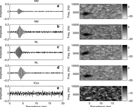
The spike-triggered average (STA) is computed by averaging the PESE across spikes, and gives the average stimulus preceding a spike. For auditory stimuli, the STA is only non-negligible in the case where there is precise synchronization to the stimulus; in particular, the neurons must display phase-locking (Eggermont 1993). Consistent with reports of phase-locking in NM (K¨oppl 1997b) and in NL (Carr and Konishi 1990; Pe˜na et al.1996), we saw coherent STAs in these nuclei for all neurons examined (fig. 3.2a–d). In ICcc, neurons do not phase-lock, and as anticipated, the STAs of ICcc neurons lacked coherent structure (fig. 3.2e).

−0.5 0 0.5 NM Amplitude

a

b

c

d

0 5 10 15 20

−0.2 0 0.2 ICcc Precedence (ms) Amplitude

e

5 10 15

5000 10000

−20

−10

Figure 3.2. Shown are the spike-triggered averages of example NM (a–b, left column), NL (c–d), and ICcc (e) neurons, along with their spectrograms (right column). The abscissa gives the time preceding the spike; color bars are provided for reference, but in following figures will be omitted a: 2003Oct31-863.06, 6,614 spikes;b: 2003Nov28-863.07, 5,234 spikes;c: 2005Feb18-854.02, 2,984 spikes;d: 2005Mar11-813.02, 3,509 spikes;e: 2005Jun08-842.03, 3,468 spikes.

given by the alternation of those bands, regardless of the actual value of the stimulus att,

a

Precedence (ms)

Precedence (ms)

6 8 10

6 7 8 9 10

100 200 300 400 0 0.05 0.1 0.15 0.2 Eigenvalue rank Eigenvalue

b

0 10 20

−0.2 −0.1 0 0.1 0.2 Precedence (ms) Amplitude

c

e

5 10 15 2000

4000 6000 8000 10000

0 10 20

−0.2 −0.1 0 0.1 0.2 Precedence (ms) Amplitude

d

f

5 10 15 2000

4000 6000 8000 10000

Figure 3.3. The spike-triggered covariance of the ICcc neuron shown in fig. 3.2e. a: The covariance matrix itself is shown. The diagonal of the matrix gives the variance, which tends to dominate over the covariance. To emphasize the covariance structure, the central 40 μs along the diagonal have been zeroed out for this plot only (thus, the band of gray along the diagonal represents zero; black positive values, white negative values). The rippling pattern of the covariance is now visible. b: The first four hundred eigenvalues of the covariance matrix, sorted by magnitude. It can be seen that the first two eigenvectors are distinct from the smooth progression seen in the remaining values. c andd: The eigenvectors corresponding to the first and second eigenvalues, respectively. Note their structure is similar to the structure of the STAs in fig. 3.2. e andf: The corresponding spectrograms of the eigenvectors.

The STC is difficult to visually interpret, and since the tuning is limited to a certain range of time, it contains an excess of data. To deal with this, we used principal component analysis, determined the significant eigenvectors of the matrix, and used only those eigenvectors in our analysis (see Methods; fig. 3.3b–f). Of the 27 ICcc neurons examined, 24 displayed at least one significant covariance eigenvector, and 18 of those had two.

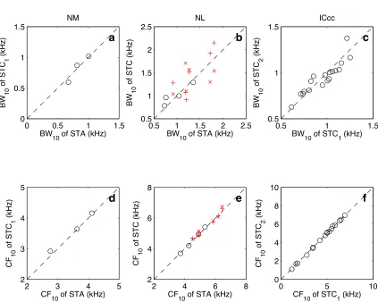
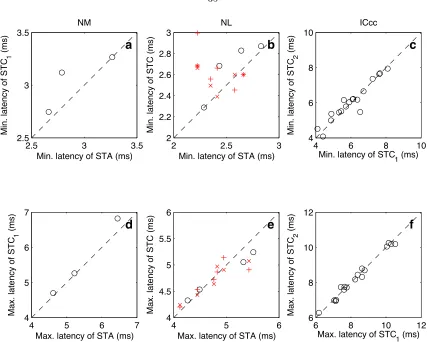
examined, 3 had a single significant covariance eigenvector. Of the 19 NL neurons, 10 had at least one significant covariance eigenvector, and 6 of those had two. To understand why multiple filters (either the STA with STC eigenvectors, or STC eigenvectors alone) are present, we note that Yamada and Lewis (1999) demonstrated in the bullfrog’s auditory nerve that non-phase-locked responses were described by pairs of filters. These pairs, called quadrature pairs, were identical in spectral profile but shifted ninety degrees in phase with respect to each other. A quadrature pair forms a basis with which all possible signals with the same spectral profile but different phases can be generated. Different weightings of the filters will produce different phase biases in the response. Even neurons with a high degree of phase-locking will respond to a wide range of phases (Johnson 1980; Carr and Konishi 1990; K¨oppl 1997b). Thus, depending on the nature and quality of phase-locking for a single neuron, a quadrature pair of an appropriate bias may be required to describe the response. When we compare the spectral profiles of the neurons with two filters (STA and the first STC eigenvector (STC1) for NL and NM, and STC1 and the second STC eigenvector (STC2) for ICcc), we see that they are similar (fig. 3.4). Equally important is determining that their temporal profiles are similar, and the latencies of the appropriate filters are in fact well correlated (fig. 3.5). Estimations of the phase differences further confirm that the filters are separated by approximately ninety degrees (NM: 91±5.7◦; NL: 89±7.9◦; ICcc: 97±27◦), confirming that when only two filters are present, they approximately form a quadrature pair.

The quadrature pair hypothesis does not predict the possibility of a third filter. However, it is clear that while the CF10of the respective filters are the same (fig. 3.4b), the BW10 (fig. 3.4e) and the latency (fig. 3.5b,e) do not show the same similarity as seen in the cases where there are only two filters. This point will be examined in further detail in the Discussion. Excepting this case, however, we observe that multiple filters are generally differentiated only by their phase. Since the majority of our analyses do not focus on phase, from this point forward we will primarily refer only to a single filter, and refer to that as the STRF.

0 0.5 1 1.5 0 0.5 1 1.5

a

10 of STA (kHz)

BW 10 of STC 1 (kHz) NM

2 3 4 5

2 3 4 5

d

CF₁₀ of STA (kHz)

CF

10

of STC

1

(kHz)

0.5 1 1.5 2 2.5 0.5 1 1.5 2 2.5

b

10 of STA (kHz)

BW

10

of STC (kHz)

NL

2 4 6 8

2 4 6 8

e

CF₁₀ of STA (kHz)

CF

10

of STC (kHz)

0.5 1 1.5

0.5 1 1.5

c

BW

10 of STC1 (kHz)

BW 10 of STC 2 (kHz) ICcc

0 5 10

0 2 4 6 8 10

f

CF₁₀ of STC₁ (kHz)

CF

10

of STC

2

(kHz)

Figure 3.4. a: When the BW₁₀for the STA and the first eigenvector of the STC (STC₁) are plotted against each other for NM, we see a generally linear relationship, though the paucity of data makes this conclusion tenuous. This is true when the same is plotted in NL for neurons with only STC₁ significant (b,◦). The dispersion is greater for the NL neurons which had two significant eigenvectors (STA vs STC₁: ×; STA vs STC₂: +). c: The BW₁₀ of STC₁ and STC₂ for ICcc neurons with two significant covariance eigenvectors. Again, a good correspondence in the majority of cases is observed (regression: r2 = 0.83, p < 10−6. d–f: The CF₁₀ in all cases showed a high degree of correspondence between filters (symbols as in a–c; regression for ICcc: r2 = 1.00, p < 10−6.). Regression values are not given for NM and NL due to lown.

neuron (fig. 3.6b; regression for maximum latency: r2 = 0.77, p <10−6; regresssion for minimum latency: r2= 0.66,p <10−5). On the other hand, while the correlation is present in NL, it is weaker (fig. 3.6a; regression for maximum latency: r2 = 0.62,p < 10−4; regression for minimum latency: r2= 0.26,p >0.01). Latencies in NM were entirely uncorrelated with frequency (p >0.01 for both cases; data not shown).

2.5 3 3.5 2.5

3 3.5

a

Min. latency of STA (ms)

Min. latency of STC

1

(ms)

NM

4 5 6 7

4 5 6 7

d

Max. latency of STA (ms)

Max. latency of STC

1

(ms)

2 2.5 3

2 2.2 2.4 2.6 2.8 3

b

Min. latency of STA (ms)

Min. latency of STC (ms)

NL

4 5 6

4 4.5 5 5.5 6

e

Max. latency of STA (ms)

Max. latency of STC (ms)

4 6 8 10

4 6 8 10

c

Min. latency of STC

1 (ms)

Min. latency of STC

2

(ms)

ICcc

6 8 10 12

6 8 10 12

f

Max. latency of STC

1 (ms)

Max. latency of STC

2

(ms)

Figure 3.5. Comparison of minimum latency for paired filters in NM (a), NL (b), and ICcc (c; regression: r2 = 0.90, p < 10−6), with symbols as in figure 3.4. The two-filter cases are generally well correlated; though some deviations are seen in NM and NL, the overall range of values is quite small. The maximum latencies (d–f) were well correlated in all cases (regression for ICcc: r2= 0.98, p <10−6; again, regression values for NM and NL are not provided due to lown).

dependence was seen (p < .001) for the STA (fig. 3.7b). Segregating the NM and ICcc populations by the number of filters did not affect this result. This stands in contrast to the observation that in NM (K¨oppl 1997a) and in ICcc (fig. 3.8) estimates of frequency tuning bandwidths using single-tone methods reveal such a dependence.

30002 4000 5000 6000 7000 2.5 3 3.5 4 4.5 5 5.5 6 NL

CF₁₀ of STA (Hz)

Latency of STA (ms)

a

0 2000 4000 6000 8000 4 5 6 7 8 9 10 11 ICcc

CF₁₀ of STC₁ (Hz)

Latency of STC

1

(ms)

b

Max. latency Min. latency

Figure 3.6. a: In NL, a linear relationship between maximum latency (◦) and CF10 was observed (r2 = 0.62, p < 10−4). The correlation for minimum latencies was not significant (+; p >0.01); as can be seen, the slope of the minimum latencies is almost zero. Both minimum and maximum latencies in ICcc showed a strong linear dependence on CF₁₀ (b; maximum latency: r2 = 0.77, p <10−6; minimum latency: r2 = 0.66, p < 10−5). No relationship was seen for latencies in NM (data not shown).

3.2.2

Effect of ITD on STRF

The neurons of both NL and ICcc are known to be tuned to ITD, which is a function of the position of the signal in space. The data on STRFs we have shown was collected at the CD alone. It is reasonable to ask what, if any, effect ITD has on the STRF properties. When we collected the reverse correlation, we interleaved trials using a second ITD to prevent habituation. These second ITDs were chosen so that across the entire set of neurons collected they covered a variety of different ITD conditions, including favorable (a peak on the ITD tuning curve other than CD), unfavorable (a trough on the ITD tuning curve), and intermediate values. In ICcc we rarely chose unfavorable ITDs, as they generally had firing rates that were too low to collect a sufficient number of spikes for reverse correlation.

2000 3000 4000 5000 600 700 800 900 1000 1100

a

10 (Hz)

BW

10

(Hz)

NM

3000 4000 5000 6000 7000 500 1000 1500 2000 2500

b

10 (Hz)

NL

0 2000 4000 6000 8000 600 800 1000 1200 1400 1600 1800

c

10 (Hz)

BW

10

(Hz)

ICcc

NM NL ICC

600 800 1000 1200 1400 1600 1800 2000

d

Figure 3.7. Plots of BW₁₀ vs. CF₁₀ for NM (a), NL (b), and ICcc (c). Both in NL and NM there is an dependence of BW₁₀ on CF₁₀, while in ICcc no such relationship is apparent. d: Distribution of BW₁₀ in the three nuclei. The bandwidths observed in NM are significantly lower than seen in either NL or ICcc (see text). Removal of the three apparent outliers ina does introduce a linear relationship (p <0.01), but examination of those neurons gives no grounds for exclusion. Removal of the outlier inchas no effect.

1000 2000 3000 4000 5000 6000 7000 200

400 600 800 1000 1200 1400 1600 1800

F 50 (Hz)

W 50

(Hz)

Figure 3.8. A linear relationship is observed between F50and W50when frequency is estimated using an iso-intensity frequency tuning curve in ICcc (regression: 0.18x+ 237 Hz, r2= 0.55,p <10−4).

3.2.3

Separability

2000 4000 6000 8000 2000 4000 6000 8000

NL

CD CF₁₀

Non−CD CF

10

a

0 1000 2000 3000

0 1000 2000 3000

CD BW₁₀

Non−CD BW

10

b

3 4 5 6

3 4 5 6 CD Latency Non−CD Latency

c

0 2000 4000 6000 8000 10000 0

5000 10000

CD CF₁₀

Non−CD CF

10

d

500 1000 1500

500 1000 1500

CD BW₁₀

Non−CD BW

10

e

6 8 10 12

6 8 10 12 CD Latency Non−CD Latency

f

ICcc

Figure 3.9. STRFs were estimated for all non-CD ITDs collected, and the CF10 (a, d), BW10 (b, e), and maximum latencies (c,f) were estimated using those STRFs and then plotted against the corresponding values for the STRF of that neuron as estimated at CD. In NL (a–c), all parameters showed a strong linear dependence (a: r2 = 0.99; b: r2 = 0.82; c: r2 = 0.93; p < 10−6 in all cases). In ICcc, a correlation was also obvious, though weaker in the case of BW₁₀ (d: r2= 0.1;e: r2= 0.54;f: r2= 0.91;p <10−6ford andf,p <0.001 fore).

apparently small, with most of the difference occurring in regions that seem to lack tuning.

a

2000 4000 6000 8000 10000

b

c

d

Frequency (Hz)

e

f

g

2 4 6 8

2000 4000 6000 8000 10000

h

Precedence (ms)

2 4 6 8

i

2 4 6 8

Figure 3.10. a: Spectrogram of the STA for an example NM neuron. b: Reconstruction of the STA’s spectrogram using the first singular vector pair. c: Reconstruction using the first two singular vector pairs. d–f andg–i are the same for the STA of a NL and the STC₁of an ICcc neuron, respectively. The tapers of the tuning become more pronounced with the added singular vector pair.

0 20 40 0

10 20 30 40 50

a

Fractional Energy (%)

NM

0 20 40

0 20 40 60

b

Singular value rank NL

0 20 40

0 10 20 30 40

c

ICcc

Figure 3.11. Fractional energy of the singular values of the STA (for NM (a) and NL (b)) and STC1 (for ICcc;c) for all neurons.

d, g). However, even the second component lacks this bias, with the power between the two regions having no significant difference (fig. 3.12b, e, h). Even when the summed activity of singular vectors other than the first is considered there is no indication of preferential action within the tuned region (fig. 3.12c, f, i). Taken all together, this suggests that there is no reason to believe that the observed inseparability reflects a significant interaction between frequency and tuning in the STRF.

3.2.4

Variability

The temporal profiles of the filters as shown in this research are narrow (figs. 3.2, 3.3). This indicates that the lag between the stimulus matching the STRF of the neuron and the spike time is relatively fixed across reoccurences of the preferred stimulus. Alternatively, we expect that the neurons of these nuclei would display low variability, and demonstrate similar responses for repeated presentations of the same stimulus. We tested this directly in 10 NL neurons and 22 ICcc neurons. As seen in figure 3.13a, b, the spike rasters are indicative of a fixed pattern of firing.

Tuned Untuned 0 0.5 1

a

b

c

Fraction of total power

d

e

f

g

h

i

Figure 3.12. a: Comparison of fractions of power in the first singular value of the STRFs for NM neurons in the tuned and untuned regions. b: The same for the second singular value. c: The comparison for the summed activity of all singular values but the first. Similarly for NL (d–f) and ICcc (g–i). Boxes extend from lower quartile to upper quartile of the sample, with the line marking the median. Outliers (+) are data points greater than 1.5 times the interquartile range of the sample.

0 50 100 150 50 100 150 200 250 Time (ms) Trial number NL

a

0 50 100 150

50 100 150 200 250 Time (ms) ICcc

b

−2 −1 0 1 2

0 5 10 15 20

Normalized # coincidences

Delay (ms)

c

−2 −1 0 1 2

0 2 4 6 8 10 12 14 Delay (ms)

d

Figure 3.13. Example spike rasters for a NL (a) and ICcc (b) neuron, using repeated presentation of identical broadband stimuli. candd: The respective SACs fora andb. Note the fine-time scale modulation of the NL SAC, which arises due to the phase-locking of the neuron, is absent in the ICcc SAC. Despite that, their outer half-height widths are similar.

3.3

Discussion

NL ICcc 0.4

0.6 0.8 1 1.2 1.4

SAC half−height width

a

NL ICcc

2 4 6 8 10 12 14 16 18

SAC height

b

Figure 3.14. a: The half-height widths of the SACs for NL and ICcc neurons. b: The maximum height of the SACs for NL and ICcc neurons.

to more complex ones. Our study was done using different techniques, but the STRFs we describe in ICcc are similar to the simpler of the STRFs that they describe. While this does not rule out a contribution from the ILD pathway, it must be noted that STRFs have yet to be demonstrated within the ILD pathway.

The existence of three filters in some NL neurons is not immediately intuitive. The simplest explanation is the one alluded to in the results above: NL neurons do not phase-lock equally well to all frequencies to which they respond. Since elimination of phase-locked responses requires two filters, the presence of a frequency that elicits a non-phase-locked response necessitates the addition of a third filter. While we did not observe any such similar effect in NM, the fact that we see a broadening of STRF bandwidth from NM to NL accounts for this. Another possibility arises from the mechanics of an NL neuron. While this study treats the N