The Information in Aggregate Data

The Information in Aggregate Data

David G. Steel, Eric J. Beh, Ray L. Chambers

Abstract

Ecological analysis involves using aggregate data for a set of groups to make

inferences concerning individual level relationships. Typically the data available for

analysis consists of the means or totals of variables of interest for geographical areas,

although the groups can be organisations such as schools or hospitals. Attention has

focused on developing methods of estimating the parameters characterising the

individual level relationships across the whole population, but also in some cases the

relationships for each of the groups.

Applying standard methods used to analyse individual level data, such as linear or

logistic regression or contingency table analysis, to aggregate data will usually

produce biased estimates of individual level relationships. Thus much of the effort in

ecological analysis has concentrated on developing methods of analysing aggregate

data that can produce unbiased, or less biased, parameter estimates. There has been

less work done on inference procedures, such as constructing confidence intervals and

hypothesis testing. Fundamental to these inferential issues is the question of how

much information is contained in aggregate data and what evidence such data can

provide concerning important assumptions and hypotheses.

The Information in Aggregate Data

David G. Steel†, Eric J. Beh†and Ray L. Chambers‡ † School of Mathematics and Applied Statistics,

University of Wollongong, Wollongong, NSW, 2522,

Australia.

‡ Department of Social Statistics, University of Southampton,

Southampton, S017 1BJ, United Kingdom.

1.1 Introduction

Ecological analysis involves using aggregate data for a set of groups to make inferences concerning individual level relationships. Typically the data available for analysis consists of the means or totals of variables of interest for geograph-ical areas, although the groups can be organisations such as schools or hospitals. Attention has focused on developing methods of estimating the parameters char-acterising the individual level relationships across the whole population, but also in some cases the relationships for each of the groups.

for likelihood based inference, including hypothesis testing. In Section 3 we il-lustrate how the approach applies in the case of data from several 2 2 tables. We also consider the information contributed by aggregate and individual information when both are available in Section 4. Section 5 gives empirical results based on some real data, illustrating the loss of information due to aggregation and how hypothesis testing and analysis of residuals can be done using aggregate data. Section 6 provides a brief discussion.

1.2 Information Lost by Aggregation

Suppose that we have individual level datad

1, which has associated probability

function f

1 d

1;ψ

. The vectorψcontains the parameters of the distribution

of the individual level data. Likelihood inference about the parameter vectorψ

would be based on the likelihoodL

1 ψ

;d

1

f

1

d

1

;ψ or the associated

log-likelihood

l

1 ψ;d

1

logL

1 ψ;d

1

The score function forψ based ond

1

is

sc

1 ψ

;d

1 ∂

∂ψl

1 ψ

;d

1

(1.1)

Maximum likelihood estimates (MLEs) would usually be obtained by solving

sc

1 ψ;d

1

0 (1.2)

resulting in the MLE ˆψ.

For inference based on the MLEs we would also be interested in the (observed) information matrix

info

1 ψ

;d

1

∂

∂ψsc

1 ψ

;d

1

∂2

∂ψ∂ψTl

1

ψ;d

1

(1.3)

The expected information is

Info

1 ψ

;d

1

E info

1

ψ

;d

1

The expectation is over the distribution ofd1

. Under several regularity condi-tions the variance matrix of the asymptotic distribution of ˆψ is Info

1

1

(see for example Cox and Hinkley, 1974, Chapter 9).

Suppose we are interested in testing the hypothesis H₀. Let ˆψ0be the MLE ofψ

under H₀. There are three common approaches to testing H₀.

1. Likelihood Ratio Test (LRT) is based on the likelihood ratio

R

1

L

1 ˆ ψ0;d

1

L

1ψˆ;d

1

and

2logR

1

2l

1 ψˆ;d

1

l

1 ψˆ

0;d

1

is tested against theχ2

qdistribution withq dim ψ dim ψ0 .

2. Wald Test is based on

W

1

ψˆ ψˆ

0 T

Info

1 ψˆ;d

1

ψˆ ψˆ

0

3. Score Test is based on

ST

1

sc

1 ψˆ

0;d

1

T

Info

1 ψˆ

0;d

1

1

sc

1 ψˆ

0;d

1

The score test does not require the calculation of ˆψ, only ˆψ₀, which in some situations will be an advantage over the Wald test. However, the Wald test does not require inversion of the information matrix. All these tests may be used to produce confidence regions forψ. Efron and Hinkley (1978) argue that it is preferable to use the observed rather than the expected information matrix for inference. We will follow this approach.

Instead of individual level data we have available the aggregate datad

2

. Let

f

2

d

2

;ψ denote the associated probability function. Likelihood based

infer-ence can then be undertaken usingf

2

. In general, derivingf

2

fromf

1

may be difficult. Sincef

2

is derived from f

1

it will depend on the same parameters as

f

1. However, not all these parameters may be identifiable using aggregate data.

We assume that the individual level data set comprisesnindividuals divided into

mgroups. In general, thenindividuals are obtained from a sample of individuals,

S

1

, and the sample ofmgroups isS

2

. The sample of individuals in groupgisSg.

An important special case is when the samples are the entire finite population, i.e.

S

1

U

1

,S

2

U

2

andSg Ug. We will assume that any sampling involved

is ignorable, for example simple random sampling.

which data are unobserved or reduced and aggregation is also a process that leads to the observed data being reduced. The basic results of Breckling et al. (1994) can then be applied to examine the effect of using aggregate data.

Let sc

2 ψ;d

2

and info

2 ψ;d

2

be the score function and observed

in-formation matrix based ond

2

. The key results of Breckling et al. (1994) are

sc

2

ψ

;d

2

Esc

1 ψ

;d

1

d

2

(1.5)

info

2 ψ

;d

2

Einfo

1

ψ

;d

1

d

2

Varsc

1 ψ

;d

1

d

2

(1.6) The expectations in (1.5) and (1.6) are over the distribution ofd

1

conditional on

d

2

, that is the individual level data given the aggregate data. Hypothesis testing can also be done using this score function and information matrix as well as the likelihood based ond

2

.

In some cases using (1.5) to obtain the score function may be more convenient than direct differentiation ofl

2

logf

2

. Result (1.6) is the key to determining the information loss due to the use of aggregate data. The variance-covariance matrix of the individual level score function conditional ond

2

can be interpreted as the loss of information due to aggregation. In Section 3 we will illustrate this approach for the case ofm2 2 tables, but the result can be applied in general.

1.3 Several 2 2 Tables

1.3.1 Data Available

Suppose that the individual level data consists ofm2 2 tables giving the frequen-cies associated with two dichotomous variables,Y andX. Table 1.1 illustrates the data for groupg.

X/Y Y 1 Y 0 Total

X 1 n11g n12g n1 g

X 0 n

21g n22g n2g

Total n1g n2g ng

It is assumed that the marginal frequencies forXare fixed, or conditioned upon, and that the values ofY are independent givenX. Hence, for groupg

n_11g

Bin n

1g π1g

n

21g

Bin n

2 g π2g

whereπ1g Prob Y 1X 1! andπ2g Prob Y 1X 0! for groupg. The

associated odds ratio is

θg

π1g

1 π1g

1 π2g π_2g

Let d

1 g #" n

11g n1g n 1g ng

$ be the individual level data for groupg and

d

1 " d

1

g g

% S

2

$ be the entire individual level data set. In ecological

infer-ence the individual level data are not available, so then_11gvalues are not available. However, the marginal frequencies andngare available giving the aggregate data

d

2 g &" n

1g n1g ng

$ for groupgandd

2 &" d

2

g g

% S

2

$ for themgroups.

1.3.2 Analysis Using Individual Level Data

Letφg

π1g π2g

T

andψ#'φ T

1)(*(*( φ T

m+

T

. If no assumptions are made con-cerning the parametersφg, each table could be analysed separately with individual level data. The likelihood forφgbased ond

1

g is denotedL

1

g φg

;d

1

g and the

log-likelihood is

l

1

g

φg;d

1

g n11glogπ1g

, n12glog

1 π1g

, n21glogπ2g, n22glog

1 π2g

The individual level score function forφgis

sc

1 φg

;d

1

g

-.

/

n_11g

n₁

0gπ1g

π_1g1

1

π_1g2 n

01g

n_11g

n₂

0gπ2g

π_2g1

1

π_2g2 354

6 (1.7)

The resulting MLEs are ˆφg πˆ

1g

ˆ

π_2g T

n_11g

n₁

0g

n 01g

n_11g

n₂

0g

T

info

1 φg;d

1 g -. . . . /

n_11g

1

1

2π_1g287

n₁

0gπ

2 1g

π2 1g1

1

π_1g2

2 0

0 1

n 01g

n_11g

291

1

2π_2g287

n₂

0gπ

2 2g

π2 2g1

1

π_2g2

2 354 4 4 4 6 (1.8)

and the expected information matrix is

Info

1 φg;d

1 g -. / n₁ 0g

π_1g1

1

π_1g2

0

0 n20g

π_2g1

1

π_2g2 354

6 (1.9)

It may be of interest to test whether there is evidence that the tables are homo-geneous with respect to the conditional probabilities, i.e.π_1g π1,π2g π2for

g% S

2

, which can be written asφg φ π

1 π2

T

for allg% S

2

. This hypoth-esis may be of substantive interest or it may be convenient for further analysis and interpretation. For example, if we have a sample of groups then assuming group specific parameters means that no inferences can be made concerning groups that are not in the sample. Even if all groups in the population of interest are included inS

2

, the large number of groups may make interpretation of the analysis dif-ficult if each group is assumed to have different parameter values. One approach to this issue is to allow for variation inφg by including random effects, but for non-linear models, this introduces considerable complexities in the analysis.

Ifφg φ, then the log-likelihood forφbased ond

1 is l 1 φ ;d 1

∑

g: S;

2<

l

1

g φ

;d 1 g n11

logπ1, n12

log1 π1

, n21

logπ2, n22

log1 π2

Hence the tables can be collapsed and the analysis can be based on the 2 2 table for the entire sample,S

1

. The MLEs, score and information functions are as in (1.7), (1.8) and (1.9) with the gfor the elements of d

1

replaced with the summation subscript= . That is

sc 1 φ ;d 1 -/ n₁₁ 0 n₁

0>0π1

π₁ 1

π₁! n

010

n₁₁

0

n₂

0>0π2

π₂ 1 π₂!

3

info 1 11 φ ;d 1 n₁₁ 0 1

2π₁!

7 n₁ 0>0π 2 1 π2 1 1

π₁!

2

info

1

21

φ;d

1 0 info 1 22 φ ;d 1 n 010

n₁₁

0

!? 1

2π₂!

7 n₂ 0>0π 2 2 π2 2 1

π₂!

2 @A A A AB A A A A C (1.11)

The resulting MLEs are ˆφ n11 0 n₁ 0>0 n 010

n₁₁ 0 n₂ 0>0 T .

The hypothesisφg φcan be tested using the likelihood ratio, Wald or score test.

The latter two can be based on the observed or expected information matrix. Also the likelihood can be directly examined to see what evidence it provides (see Roy-all, 1997). For example, when the tables are homogeneous,ψ0D'φ

T E(F(*() φ

T

+

T

and the score test using the observed information matrix is

ST

1

∑

g: S

;2 < sc 1 φˆ ;d 1 g T info 1 φˆ ;d 1 g 1 sc 1 φˆ ;d 1 g

∑

g: S

;2

<

ST

1 g

The likelihood ratio is

R

1

∏

g: S;2

<

L

1

g ˆ

φ;d

1

g

L

1

g ˆ

φg;d

1

g

∏

g: S;2

<

R

1 g

1.3.3 Analysis Using Aggregate Data

In ecological inference the data available from each table are d

2

g so that n11g

is not available. We could attempt an analysis without making any assumptions concerningφg. This amounts to analysing each group separately. Applying (1.5) to (1.7) immediately gives

sc

2 φg;d

2 g -. . . / E1

n_11g

G

d;2

<

g 2

n₁

0gπ1g

π_1g1

1

π_1g2 n

01g

E1

n_11g

G d; 2< g 2 n₂

0gπ2g

π_2g11

π_2g2

354

4

4

6

Conditional ond

2

g ,n11ghas a non-central hypergeometric distribution (see for

E

n_11gd

2 g

P₁ θg;d

2

g

P₀ θg;d

2

g

where

Pr θg;d

2

g !H

bg

∑

jI ag

J

n₁g

j K

J

n₂g

n

1g jK

jrθj g

The limits of the sum are the lower and upper bounds onn_11ggivend

2

g and are

ag max

0 n 1g n2

g

andbg

min

n₁g n1g

. Denote E

n_11gd

2

g by

κ1 θg;d

2 g . Also

Var

n_11gd

2

g

P₂ θg;d

2

g

P₀ θg;d

2

g

κ

1 θg

;d

2

g

2

which will be denoted byκ2 θg;d

2

g .

From (1.7) Var sc 1 φg ;d 1

g d

2

g κ

2 θg

;d 2 g -. / 1 π2 1g1

1

π_1g

2

2

1

π_1gπ_2g1

1

π_1g291

1

π_2g2

1

π_1gπ_2g1

1

π_1g2L1

1

π_2g2

1

π2 2g1

1

π_2g2

2

354

6

Applying (1.6) with (1.7) and (1.8) gives

info 2 11 φg ;d 2 g κ₁ θg;d

2

g

1 2π

1g

,

n₁

gπ

2 1g κ

2

θg;d

2

g

π2

1g

1 π

1g 2 info 2 21 φg ;d 2 g

κ₂ θg;d

2

g

π_1gπ_2g

1 π

1g

1 π

2g info 2 22 φg ;d 2 g n 1g κ

1 θg;d

2 g 1 2π 2g , n2

gπ

2 2g κ

2 θg;d

2 g π2 2g

1 π

2g

Setting sc

2 φg;d

2

g 0 yields the relationship π_1gn₁g, π2gn2g

n

1g

or

π_2g

n 1g

n₂g

n₁g

n₂g

π_1g (1.12)

which corresponds to the tomography line for groupgdiscussed in King (1997, pg 80) .

The aggregation of the data has resulted in each element of the information ma-trix being modified by a term proportional toκ₂ θg;d

2

g arising from the

con-ditional variance of the individual level score function. Alson_11gis replaced by its expectation conditional ond

2

g .

For each group there is only one observed random variable,n

1g

and two pa-rameters unless some further assumptions are made. Formgroups there are m

observations,n

1g

,g% S

2, but 2mparameters. Hence standard asymptotic

prop-erties of likelihood based methods cannot be relied upon. Beh, Steel and Booth (2002) consider the likelihood associated with aggregate data for a single group. This is given by McCullagh and Nelder (1989, pg 353) :

L

2

g

φg;d

2

g

1 π1g

n₁

0g πn01g

2g

1 π2g

n₂

0g

n 01g

P₀ θg;d

2

g (1.13)

Wakefield (2001) uses the same likelihood, but presents it in the form of a convo-lution likelihood of two binomials.

Beh, Steel and Booth (2002) show that the likelihood surface has a ridge along the tomography line (1.12). Along the tomography line the likelihood is minimised whenπ_1g π

2g, i.e. at independence, and the maximum occurs at one of the

ends of the tomography line. They also show that except for cases whenn1g

is very close ton₁gorn2gthe likelihood surface is not able to provide useful

evidence concerning the values ofπ_1gandπ_2gother than they should be on the tomography line. Notice that the score and information function in this case can also be obtained directly from the likelihoodL

2

g given by (1.13).

Beh, Steel and Booth (2002) obtain the exact values of ˆφg ˆ

π1g

ˆ

π2g T

that maximise the likelihood. Wakefield (2001) also obtains these values using an ap-proximation. The resulting maximum of the likelihoodL

2

g φgˆ;d

2

g can also be

obtained. Notice ˆφgis unique, except whenn₁g n2

g, in which case the

likeli-hood is maximised at 0 1

!

T _{and 1}

0

!

T_.

mobservations can be tackled if we assumeφg φ for all g% S

2

. Of course this is a very strong assumption and it is more realistic to assume thatφgvaries in some way across them groups. The variation may be related to group level covariateszgand random effects. However, analysis is relatively straight forward

if this homogeneity assumption holds. More importantly the question arises of whether, in practice, it is possible from aggregate data alone to assess whether the homogeneity assumption is reasonable before attempting to use methods that allow for variation inφg.

Whenφg φ, we can obtain the score and information functions based on the

aggregate data for themgroups in the sample by applying (1.5) and (1.6) to (1.10) and (1.11) or summing the score and information functions arising from each group withφg φ. This gives

sc

2 φ;d

2

-.

/

∑gκ₁ θ;d;2

<

g !

n₁

0>0π1

π₁ 1

π₁! n

010

∑gκ1 θ;d;2

<

g !

n₂

0>0π2

π₂ 1

π₂!

34

6

info

2

11

φ;d

2

∑gκ1 θ

;d

2

g

1 2π

1

, n1Mπ

2 1 ∑gκ

2 θ

;d

2

g

π2 11

π

1

2

info

2

12

φ

;d

2

∑gκ2 θ;d

2

g

π₁π₂1

π

1N1

π

2

info

2

22

φ

;d

2

n1

∑gκ1

θ;d

2

g

1 2π2

, n2Mπ

2 2 ∑gκ2

θ;d

2

g

π2

2 1 π2

2

Setting sc

2 φ

;d

2

0 gives the overall sample level tomography line

π₁n₁M, π2n2M

n

1

The correlation between the two elements of the individual level score function conditional ond

2, obtained from Var sc

1 φ;d

1

d

2

, is 1 and

corre-sponds to the constraint arising from the tomography line. Comparing info

2

with info

1

we see that in addition to the reduction in the diag-onal elements, a positive term appears in the off-diagdiag-onal elements. This suggests that inferences concerningπ₁ π2will be particularly badly affected.

L

2 φ;d

2

∏

g: S;

2<

L

2

g

φ;d

2

g

McCullagh and Nelder (1989, pg 353) obtain an equivalent score function for a different parameterisation.

The equations sc

2 φ

;d

2

O 0 can be solved to obtain the estimates ˆφ

πˆ

1

ˆ

π₂ T

under the hypothesis of homogeneity. This can be done in several ways as reviewed by Beh and Steel (2002). Here we obtain the estimate ofφ using the Newton-Raphson iterative procedure

φ j 7 1 φ j αA 1 J ∂l ∂φKQP P P P

φI φ;j

<

with the secant approximation of hessian matrixAto accelerate convergence. Red-dien (1986) comments that the use of this approximation is often preferred to the standard Newton-Raphson procedure and that its rate of convergence is both sat-isfactory and stable. The value ofαis chosen such that 0R α R 1 and dictates the

step length taken at iteration of the procedure (see McCulloch and Searle, 2001, pg 269).

Once an estimate of the common probabilities, ˆφ, is obtained we can produce estimates of the group specific proportionsP_1g n11g

S

n₁

g

andP_2g n21g

S

n₂

g

by evaluating the expectation En

11gd

2

κ

1 θˆ

;d

2

g where ˆθis the odds ratio

calculated from ˆφ. This gives the estimates ˆP_1g κ1 ˆ

θ;d

2

g

S n1 g

and ˆP_2g

n1g

κ

1 θˆ

;d

2

g T

S n2g. For each group these estimates of the proportions

are obtained by projecting the estimates of the common probabilities, ˆφ, onto the tomography line (1.12) for that group, using the expectation of the non-central hypergeometric distributionκ₁ θˆ

;d

2

g .

The likelihood ratio for testing the hypothesisφg φis

R

2

∏

g: S

;

2<

L

2

g φˆ;d

2

g

L

2

g φgˆ ;d

2

g

∏

g: S

; 2< R 2 g

We will not use the Wald test as info

2

is not defined at the ˆφgvalues. The score test based on the observed information matrix is

ST

2

∑

g: S;2

< sc 2 φˆ ;d 2 g T info 2 φˆ ;d 2 g 1 sc 2 φˆ ;d 2

g

∑

g: S;2

<

ST

1.4 Using Aggregate and Unit Level Data

In some situations it may be feasible to obtain both individual level and aggregate data. For example, we may have a reasonably large number of groups and could consider conducting a small sample of individuals to supplement the aggregate data. Alternatively, we could have a reasonable sized sample of individuals and consider supplementing it by some aggregate data. The latter case could be useful in producing estimates of group specific quantities. This leads to the general issue of what is the relative value of the two types of data. This can help us decide at what sample size the information in the aggregate data has little additional value. Suppose that we have a simple random sample,S

0 ofn

0individuals selected

from the population of interest. We assume that the sampling fraction is small so that we can treat the data inS

0

as independent of that inS

2

. The sampleS

0

produces the datad

0

. The aggregate and individual level data can be combined, givingd c U" d 2 d 0

$ . Because of the independence of the data sets the score

function and information matrices can be added giving

sc

c

ψ;d

c

sc

2

ψ;d

2 , sc 0

ψ;d

0 info c ψ ;d c info 2 ψ ;d 2 , info 0 ψ ;d 0

Consider the case ofm2 2 tables. Suppose that the group that each individual comes from is not known. This could be for reasons of confidentiality or because the sample was selected in a way that did not make recording the groups conve-nient. Thend

0

" n

0

11 n

0 1 n 0 1 n 0 $ .

Assumingφg φthe information associated withd

0 is info 0 11

φ;d

0 n; 0< 11 1

2π₁!

7 n; 0< 10 π2 1 π2 1 1

π₁!

2

info

0

21

φ;d

0

0

info

0

22

φ;d

0

1

n;0

<

01

n;0

<

112

1

2π₂!

7

n;0

< 20 π2 2 π2 2 1

π₂!

2 @A A A A AB A A A A A C

The addition of the unit level data increases the diagonal elements of the infor-mation matrix and leaves the off-diagonal elements unchanged. Besides reducing the asymptotic variance of the estimates ofπ₁andπ₂this will also dampen the correlation of the estimates resulting in additional benefits for the estimation of

π₁ π

1.5 Example

To illustrate the application of these results we will consider a simple example using data from the 1996 Australian census. The data corresponds to the census district (CD) level data for the city of Brisbane in Australia where the individual level classifications are known. There are a total of 1541 CDs, but for simplicity we will focus our discussion on a random sample of 50 CDs.

For comparison, King’s method is also applied to these data using the EzI package (Benoit and King, 1998) with its default global parameters.

Consider the data with variables ”Income” and ”Age” so that for CDgthe classi-fication of individuals is

X 1; if a person is aged between 15 and 24 years,

X 0; if a person is aged at least 25 years,

Y 1; if a person’s weekly income is between $AU0 and $AU159,

Y 0; if a person’s weekly income is at least $AU160.

For the 50 CDs considered there are 22323 individuals classified, with 4238 in-dividuals aged between 15 and 24 years and 5674 with a weekly income of be-tween $AU0 and $AU159. These values correspond to the marginal frequencies

n ,n1

M andn1 respectively. The proportion of people aged between 15 and

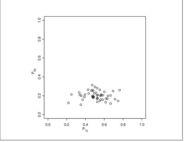
24 was 0.1898 and varied from 0.1053 to 0.2861 with a coefficient of variation 0.1970. A plot of the values of the group specific proportionsP_1gandP_2gis given in Figure 1.1 and shows a considerable amount of variation.

Based on the individual level data we obtain ˆπ

1

1 0

(5054 and ˆπ

1

2 0 (1953

which have estimated standard errors of 0.0077 and 0.0029 respectively.

Based only on the aggregate level data the maximum likelihood estimates as-suming homogeneous parameters using the accelerated Newton-Raphson iterative procedure gives ˆπ

2

1 0

(

5184 and ˆπ

2

2 0

(

1922 and estimated standard errors of 0.0353 and 0.0085 respectively. The initial values of π₁ andπ₂ were set at 0.6 and 0.1966 so that the overall tomography line is satisfied. Instability of the convergence was experienced withα 1 so smaller steps throughout the

itera-tive procedure were carried out withα 0

(4. Using King’s (1997) method via

EzI produced estimates ˜π

2

1 0

(4769 and ˜π

2

2 0

(2020 with estimated standard

errors of 0.1606 and 0.0376 respectively. The point estimates obtained from the two methods are quite similar although there is a large difference between the es-timated standard errors. This may be due to the random effects incorporated into the King method while our approach does not include any random variation in the group specific parameters.

0.0 0.2 0.4 0.6 0.8 1.0

0.0

0.2

0.4

0.6

0.8

1.0

P1g

P2g

Figure 1.1 Plot of P_2gversus P_1g

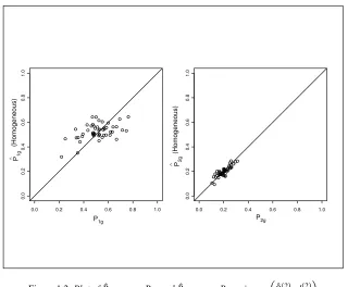
and assuming homogeneity of the associated probabilities are very similar. In the latter approach, even though the probabilities π_1g andπ_2g are assumed to be constant across the groups, the associated proportions,P_1g and P_2g are not assumed to be constant across the groups. Figure 1.2 compares the individual level proportionsP_1g andP_2gwith the estimates ˆP_1gand ˆP_2gobtained by considering the expectation En

11gd

2

g using the parameter values ˆπ

2

1 and ˆπ

2

2 , that is

κ1 ˆ

θ

2

;d

2

g . These values are very similar to those produced when estimating

P_1gandP_2gusing King’s approach and these are produced in Figure 1.3. Chambers and Steel (2001) considered using the relative root-mean-squared errors

V₁

1 ˆ

π

1

1 V

m

1

∑

g Pˆ

1g P

1g

2 V₂

1 ˆ

π

1

2 V

m

1

∑

g Pˆ

2g P

2g

2

to assess how well these estimates reproduce the true values. For the method as-suming homogeneity between the groupsV₁ 0

(

1993 andV₂ 0

(

1204, while King’s method produces the similar valuesV₁ 0

(

2066 andV₂ 0

(

0.0 0.2 0.4 0.6 0.8 1.0

0.0

0.2

0.4

0.6

0.8

1.0

0.0 0.2 0.4 0.6 0.8 1.0

0.0

0.2

0.4

0.6

0.8

1.0

P_1g P_2g

P1g

∧

P2g

∧

(Homogeneous)

(Homogeneous)

Figure 1.2 Plot ofPˆ_1gversus P_1gandPˆ_2gversus P_2gusingκ₁W

ˆ

θX

2Y;d

X

2Y

g Z

Based on the individual level parameter estimates ˆπ

1

1 and ˆπ

1

2 the information

matrix and its inverse are

info

1

J

16953(96 0

0 115075(3

K

info

1

1

J

0(00005898323 0

0 0(00000868996

K

This gives the estimated standard errorsSE[

1 πˆ

1

1 d

1

0

(0077 and

[

SE

1 πˆ

1

2 d

1

0(0029.

The conditional expectation of this information matrix can be evaluated by re-placingn_11gby its conditional expectation evaluated at ˆθ

2

. Doing so yields

E info

1 d

2

J

16991(07 0

0 117205(8

K

which is very close to info

1

0.0 0.2 0.4 0.6 0.8 1.0

0.0

0.2

0.4

0.6

0.8

1.0

0.0 0.2 0.4 0.6 0.8 1.0

0.0

0.2

0.4

0.6

0.8

1.0

P_1g P_2g

P1g

∧ ∧ P2g

(King) (King)

Figure 1.3 Plot ofPˆ_1gversus P_1gandPˆ_2gversus P_2gusing King’s Methodology

Using ˆπ

2

1 , ˆπ

2

2 and ˆθ

2

from the Newton-Raphson procedure

Varsc

1 d

2 \

J

11927

(

53 19179

(

83

19179

(83 30841(74

K

which has an associated correlation of 1. Applying (1.6) the resulting

informa-tion matrix based only on the aggregate level data is

info

2

J

5063

(

538 19179

(

83 19179(83 86364(03

K

and

info

2 ]

1

J

0(0012436897

0

(00027620009

0

(00027620009 0(00007291774

K

and so the estimated standard errors areSE[

2 πˆ

2

1 d

2

0

(0353 and

[

SE

2 πˆ

2

2 d

2

The difference in the probabilities,π1 π2 will often be of particular interest. From info 1 we obtain [ Var 1 πˆ 1

1 πˆ

1

2 d

1 [ Var 1 πˆ 1

1 d

1 , [ Var 1 πˆ 1

2 d

1

2Cov^

1 πˆ 1 1 ˆ π 1

2 d

1 0 ( 00005879863 , 0 (

000008480757 2 0

0 (00006727939 Hence [ SE 1 πˆ 1

1 πˆ

1

2 d

1 0 (008202401 From info 2 [ Var 2 πˆ 2

1 πˆ

2

2 d

2 Var[ 2 πˆ 2

1 d

2 , [ Var 2 πˆ 2

2 d

2

2Cov^

2 ˆ π 2 1 ˆ π 2

2 d

2

0

(0012436897, 0(00007291774, 2 0(00027620009

0 ( 001869008 giving [ SE 2 πˆ 2

1 πˆ

2

2 d

2

_ 0

(04323203

The estimated correlation between ˆπ

2

1 and ˆπ

2

2 obtained from info

2

is 0 (917.

Parameter Var[

2 S [ Var 1

Ind. Sample Ind. Sample Equiv. to 50 CD’s Equiv. Per CD

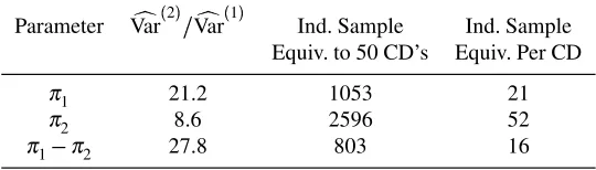
π1 21.2 1053 21

π2 8.6 2596 52

π1 π2 27.8 803 16

Table 1.2 Effect of Aggregation on Variance Estimates: Income by Age

The effect of aggregation can be examined by looking at the ratio of the estimated variances obtained from info

1

and info

2

the estimation ofπ1 is affected by aggregation more thanπ2, possibly because

π1is larger andP1gvaries more across the CDs. The increase in the asymptotic

variance of the parametersπ₁andπ₂ is more than the increase in the diagonal elements of the information matrix, i.e. more than 3.3 and 1.3 respectively. This is due to the large covariance term introduced by the aggregation. The estimation ofπ₁ π

2is affected even more than that ofπ1due to the affect of aggregation on

the correlation of the estimates. In looking at these ratios, it must be remembered that the individual level data consists of 22323 people whereas the aggregate data relates to 50 CD’s, a ratio of 446. There are 4238 people who are 15-24 years old which contribute to the estimation ofπ₁, an average of 84.8 people per CD. While there is clearly a loss of information through the use of aggregate data, it does not correspond to each CD being equivalent to an individual. In Table 1.2 we show the individual level sample size required to obtain the same variance, and therefore standard error, as using these aggregate data for 50 CD’s. For example, the sample of 50 CD’s gives the same variance for the estimation ofπ1 π2as

803 individuals. Dividing by 50 gives an indication of the information per CD compared with the information per individual. For this example, on average, each CD is as useful as 16 individuals in terms of estimatingπ1 π2. These results

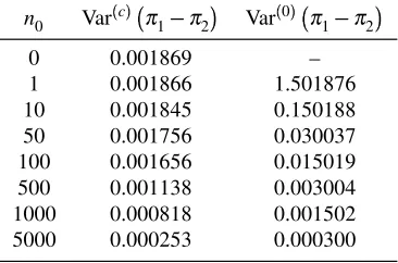
depend on the variation in the proportion of 15-24 year olds across the CD’s. Using the results in Section 1.3.4 we can also examine the likely impact of sup-plementing aggregate data with individual level survey data. This is shown in Table 1.3 which gives the variance Var

c

of the estimate ofπ₁ π

2 based on

aggregate data for 50 CD’s plus an independent sample of n₀ individuals for

n₀ 0

1

10

50

100

500

1000. For comparison, we also give the variance for these sample sizes when there is no aggregate data, Var

0

.

n₀ Var

c

π

1 π2

Var

0 π

1 π2

0 0.001869 –

1 0.001866 1.501876

10 0.001845 0.150188

50 0.001756 0.030037

100 0.001656 0.015019

500 0.001138 0.003004

1000 0.000818 0.001502

5000 0.000253 0.000300

Table 1.3 Comparison on Var`π

1a

π₂

b

for the analysis of aggregate data and a sample of individual level data of various sizes

We can also compare the use of individual and aggregate data in testing for hom-geneity, using the likelihood ratio and score test as described in Section 3, page 11. Both tests should be compared withχ2

98, for which the critical value for a 5%

test is 122.

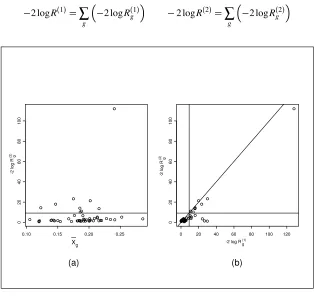
For the likelihood ratio test the results are

2logR

1

502

(7287

2logR

2

339

(2903

Both these values suggest that the null hypothesis ofφg φbe rejected. The test

statistic calculated from the individual level data is larger, which is consistent with it having more power. Each of these test statistics can be decomposed into a term for each group, i.e.

2logR

1

∑

g

2logR

1

g

2logR

2

∑

g

2logR

2

g

0.10 0.15 0.20 0.25

0

20

40

60

80

100

0 20 40 60 80 100 120

0

20

40

60

80

100

-2 log R

(2) g

-2 log R

(2) g

-2 log R(1) g X_g

(a) (b)

−

Figure 1.4 Plot of

a

2logRX

2Y

g versus Xg, anda

2logRX

1Y

g

Figure 1.4(a) gives a plot of 2logR

2

g versusXg n

1 gS

ng, the proportion of

terms of identifying groups with large values which indicates that they are par-ticularly affecting the statistical significance of the test. This will suggest those groups having parametersπ_1gandπ_2gwhich are statistically significantly differ-ent from the overall parameters values. It may also be useful in suggesting any trends in departures from homogeniety that may be related toXg.

In examining these values we suggest comparing them with the 1% critical value ofχ2

2, i.e. 9.210. The horizontal and vertical lines on the figures correspond to

this value.

Figure 1.4(b) gives a plot of 2logR

2

g versus 2logR

1

g . Of the 17 cases that

would be identified as statistically significant using individual level data, 9 are also identified using the group level data. Also no cases that are statistically non-significant using 2logR

1

g are identified as statistically significant using

2logR

2

g . Hence, while there is, as expected, a loss of power in using the

aggre-gate data, it is still possible to undertake a useful analysis of residuals.

Both the analyses of 2logR

1

g and 2logR

2

g identify one particular CD as

having a large influence on the hypothesis test. This CD was investigated and found to have more than twice the usual population size, low values ofP_1gandP_2g, and a reasonably high value ofXg. This is probably a CD in a newly developed

area of the city.

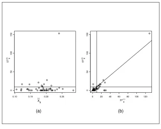
A similar approach can be used with the score test, giving

ST

1

496

(8291 ST

2

359

(9741

Figure 1.5 gives a plot ofST

2

g versusXgandST

1

g .

Again these results both lead to the rejection of the null hypothesis. However, we encountered a problem with the score test. For 24 of the 50 CDs, info

2 φˆ

;d

2

g

was not positive-definite, leading to a negative ST

2

g value. In our analysis we set

such cases to zero. Numerically this situation arises because the subtraction of the estimate of the conditional variance of the score function for the CD reduces the diagonal elements and increases the off-diagonal elements too much. We are investigating modifications to the score test to overcome this issue. Notwithstand-ing this issue usNotwithstand-ingST

2

g identifies 10 of the 15 cases thatST

1

g would identify

as having parameters statistically significantly different from the overall values. However, it also identified one case as statistically significant that was not so identified usingST

1

g .

0.10 0.15 0.20 0.25

0

50

100

150

0 20 40 60 80 100 120

0

50

100

150

ST

(2) g g

g X_g

(a) (b)

−

ST

(2)

ST(1)

Figure 1.5 Plot of STX

2Y

g versus Xgand STX

1Y

g

1.6 Discussion

We have described a general approach to clearly identify the loss of information in using aggregate rather than individual level data. LetY_idenote the value of the re-sponse variable for individuali. In many situations determining the score function and information loss through aggregation will involve determining E Y

id

2

g ,

Var

Y_id

2

g and Cov

Y_iYj d

2

g fori

j % g.

In the example of homogeneous 2 2 tables, this approach is not much simpler than direct use of the likelihood based on the aggregate datad

2

. However, equa-tion (1.6) clearly shows the informaequa-tion loss. Much of the effect of aggregaequa-tion in this case arises from the change to the off-diagonal elements of the information matrix.

The example suggests that residuals obtained from the Likelihood Ratio Test us-ing aggregate data are preferable to those obtained from the Score Test.

We are currently considering how the general approach applies in the more com-plex models, especially those including random effects to allow for the variation in group specific parameters.

1.7 References

Beh, E. J., and Steel, D. G., ”Maximum likelihood estimation and homogeneous 2c 2

ta-bles”, Preprint 3/02, School of Mathematics and Applied Statistics, University of Wol-longong, Australia, 2002.

Beh, E. J., Steel, D. G. and Booth, J. G., ”What useful information is in the marginal fre-quencies of a 2c 2 table?”, Preprint 4/02, School of Mathematics and Applied Statistics,

University of Wollongong, Australia, 2002.

Breckling, J. U., Chambers, R. L., Dorfman, A. H., Tam, S. M. and Welsh, A. H., ”Max-imum likelihood inference from sample survey data”, International Statistical Review, 62, 349–363, 1994.

Chambers, R. L. and Steel, D. G., ”Simple methods for ecological inference in 2c 2 tables,

Journal of the Royal Statistical Society A, 164, 175-192, 2001.

Cox, D. R. and Hinkley, D. V., ”Theoretical Statistics”, Chapman and Hall, London, UK, 1974.

Efron, B. and Hinkley, D. V., “Assessing the accuracy of the maximum likelihood estimator : Observed versus expected Fisher information (with discussion)”, Biometrika, 65, 457– 487, 1978.

King, G., ”A Solution to the Ecological Inference Problem”, Princeton University Press, Princeton, USA, 1997.

McCullagh, P. and Nelder, J. A., ”Generalized Linear Models”, Chapman and Hall, Lon-don, UK, 1989.

McCulloch, C. E. and Searle, S. R., ”Generalized, Linear, and Mixed Models”, Wiley, New York, 2001.

Reddien, G. W., ”Newton-Raphson methods”, Encyclopedia of Statistical Sciences, 6, 210-212, 1986.

Royall, R. M., ”Statistical Evidence : A Likelihood Paradigm”, Chapman and Hall, Lon-don, UK, 1997.

Wakefield, J., ”Ecological inference for 2c 2 tables”, Techincal Report, Department of

Statistics and Biostatistics, University of Washington, USA, 2001.

Acknowledgment