II. METHODOLOGY A. Computational Domain

Abstract—The effect of the windward turbines in a clustered wind farm has significant effects on the performance of the downwind turbines which are characterized by velocity deficit and turbulence intensity. Various published literatures concluded that for some cases the effect of the turbine wakes in VAWT clustered configuration increases the over-all performance of the clustered wind farm. In this study, the effect of varying equivalent rotor diameter spacing were investigated. There was an increase of 4.97% in a clustered turbine arrangement with 4 equivalent rotor diameter spacing and 60 degree oblique angle compared to an isolated turbine. Meanwhile, there was no detectable increase to the performance of clustered turbine arrangement of 12 rotor diameter spacing.

Index Terms—Wake, CFD, VAWT

I. INTRODUCTION

he aerodynamic interactions of turbines grouped in arrays has been becoming a major field of interest. One interesting characteristics exhibited by a group of turbines clustered in close proximity is the wake effect. For Horizontal Axis Wind Turbines (HAWT), the effect of the wake phenomenon is generally negative due to velocity deficit. The output power of turbine under the shadow of the wakes on another turbine has reduced power production due to lower wind speed. Further, increased turbulence intensity (aerodynamic wind load) induced by turbine wake shortens the lifetime of rotors [1]. The result of the study by Neustadter, et al for example showed a 10% reduction to the power output of 3 turbines with 7 rotor separation [2]. The power loss due to wake effect varies from 5 to 40%, with turbine operating setting; number of turbine rows, turbine size, wind farm terrain and atmospheric flow conditions determines the power loss [3]

The effect of turbine clustering for the vertical axis wind turbines, however, is promising. Shaheen, Abdallah, et al found out that an efficient triangular shaped three co-rotating Savonius turbine cluster arranged in close proximity enhances the average output of its three turbines by up to

J.E. Silva, B. Sc. is a M.Sc. student of the Energy Engineering Program, University of the Philippines Diliman (corresponding author, email: [email protected])

L.A.M. Danao, PhD is an Associate Professor of the Department of Mechanical Engineering, University of the Philippines Diliman (e-mail: [email protected]).

34% compared to their isolated counterparts [4]. Other turbine clustering with 9 and 27 turbine farms increased the synergistic output by 26% and 37%, respectively. Ten percent more power was obtained by Hezavah, et al to a triangular wind turbine clustered configuration with ratio between the distance to cluster turbines relative to turbine diameter (L/D) of 5 [5]. Whittlesey, et al, found out that closely spaced turbines can cause constructive interference when rotating in opposite directions [6]. Using the same fish-schooling model as Whittlesey, Bons concluded an increase of 22% in the productivity of wind turbine farm compared to isolated turbines for a network of 16 wind turbines [7].

The application of computational fluid dynamics in the field of wind flow simulation is becoming popular. CFD offers the best solution compared to other models such as momentum and vortex models and gaining popularity for analyzing complex, unsteady aerodynamics involved in the study of wind turbines [8],[9]. As mentioned by Wekesa, Danao, et al [10], findings by Castelli et al for a numerical model to evaluate energy performance and aerodynamic forces acting on a straight-bladed Darrieus VAWT proved that CFD method was able to visualize the basic physics behind VAWT, and that CFD models can be used as an alternative to wind tunnel tests.

II. METHODOLOGY A. Computational Domain

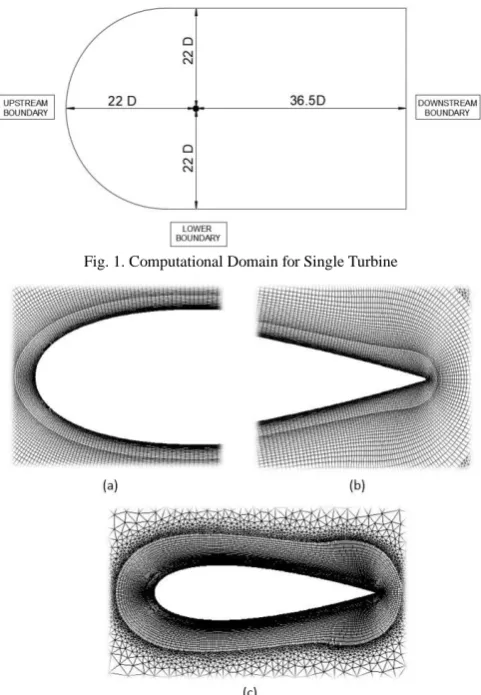
The physical characteristics of the wind farm was simulated in a computational domain composed of inner (rotating) sub-grid and outer (stationary) sub-grid. The distance of the turbines from upper and lower boundaries of the computational domain were sufficiently far to minimize boundary blockage effects and fully capture the wake development of the turbines. The computational domain used in this study is illustrated in Figure 1.

Since the stream-wise velocity component is much bigger compared to its span-wise velocity component and the wind turbine airfoils are long and slender, it is safe to assume that the flow at a given radial position is two-dimensional [11]. Essential features of the wind turbines were modelled to the mesh such as turbine blades and vertical axis hub (i.e. central hub) while the effect of radial arms was excluded in the study.

VAWT Cluster Parameter Study on Overall

Cluster Performance, Part I: Model

Development and Rotor Spacing

Jeffrey E Silva, and Louis Angelo M. Danao, Member, IAENG

Fig. 1. Computational Domain for Single Turbine

Fig. 2. Near blade mesh: (a) Leading Edge-Mesh (b) Trailing Edge-Mesh (c) Airfoil Near-Blade Mesh

(a) (b)

Fig. 3. Unstructured domain mesh (a) Rotor Mesh (b) Outer Mesh.

B. Mesh

The computational domain was divided into two domains: the stationary domain and the rotating sub-domain. The stationary sub-domain is composed of a semi-circular velocity inlet, rectangular far field boundaries and circular opening intended for the placement of the rotating sub-domain while three symmetric turbine air foil blades and hub comprise the rotating sub-domain. The rotating mesh, positioned to be coincident to the circular opening of the stationary domain, was allowed to slide and mesh with the stationary mesh at common angular speed.

The stationary sub-domain mesh was generated using

toward the external limits of the sub-domain. The total cells comprising the stationary sub-domain is about 19,000. Particular attention was given to the rotating sub-domain since most of the important flow effects happen in this region. It is very important to consider the value of the wall unit, y+ to determine the first cell height at the airfoil surface and make sure that the mesh will be able to resolve the solution at the boundary layer appropriately. Y+ is defined as the ratio between the turbulent and laminar force influences in a cell, and to capture the viscous layer the approximate value of y+ must be less than 5 [12]. Further, the CFD software also require the values of y+ to be less than 5. Different trials of grid refinement near the airfoil blade were tested to attain the target y+ for all surfaces to capture the fluid behavior at viscous sub-layer. Grid refinements were done by varying the initial step-size (i.e. first cell height) and inflating up to 25 levels of triangular cells. The rotating sub-domain has about 102,000 cells.

The airfoil blade profile was generated by importing the NACA 0025 symmetrical airfoil coordinates to the meshing software. A structured boundary layer mesh was inflated from the airfoil surface (Fig. 2) while an unstructured mesh was used to fill in the rest of the domain (Fig. 3).

C. Equiangle Skewness

A factor that influences the accuracy of the result in a CFD simulation is the cells’ equiangle skewness. Equiangle skewness, defined as the maximum ratio of the cell’s included angle to the angle of an equilateral element and ranges from 0 to 1 where 0 is the best case, tends to influence the result of the CFD simulation since values close to unity lead to numerical instabilities and inaccurate results. It is recommended that the value of the equiangle skewness should be kept below 0.8 for a good grid [13]. Shown in Fig. 4 is the mapping of the equiangular skewness of the stationary and rotating sub-domain with the highest value equal to 0.65 and 0.57, respectively. These maximum values can be found along the edges of their boundaries and might not affect the outcome of the simulation. The stationary sub-domain has an average equiangular skewness of 0.19 while the average equiangular skewness of the rotating sub-domain is 0.05.

(a) (b)

Fig. 4. Skewness values of the (a) Outer Domain and (b) Rotating Domain.

D. Turbulence Model

non-reference frames, but also the most computationally demanding.

There are many available options for modelling the turbulence behavior of this particular problem. One popular model is the k-ε model which has the advantage of simplicity in implementation and the stable calculation characteristics which generally leads to easier convergence. This model, however suffers from poor predictions in simulations involving swirling and rotating motions [14]. Further, the model requires explicit wall-damping functions and demands the deployment of fine grid spacing near solid walls. Another popular turbulence model is the k-ω model wherein k represents the turbulent kinetic energy while ω stands for the specific dissipation rate of k. This model is a modified version of the k equation found in the k-ε model and solves two partial differential equations (i.e. two-equation turbulence model). The resulting calculations for this model usually has the same numerical behavior with that of k-ε. Some advantages of the k-ω model are that this model can be applied throughout the boundary layer without further modification, it can be used without requiring the computation of wall distance and numerical stability primarily in the viscous sub layer near the wall [15]. Sensitivity to initial conditions and difficulty of convergence are the weaknesses of the k-ε model.

The above two models has its share of advantages and disadvantages. Another turbulence model capitalizes on the advantages of both the k-epsilon and k-omega model. This is the k-ω SST (Shear Stress Transport), a two-equation eddy viscosity model for CFD Flow. Known for its uniqueness, this viscosity model exploits on the versatility of the k-ω model in solving equations at the inner boundary layer which exhibits well, more robust and accurate when simulating at the inner parts of the boundary layer to the wall through the viscous sub-layer and then switches to k-ε model when solving at the outer region of and outside the boundary layer. This scheme results in highly accurate predictions on the onset and the amount of flow separation under adverse pressure gradients by including the transport effects into the formulation of the eddy-viscosity.

There was a study involving CFD numerical validation conducted by Danao, et al. In this study the authors stated that in the absence of VAWTs experimental data, the dynamic interactions of a pitching airfoil with a moving data give the closest possible validation cases versus static airfoil data. Further the paper concluded that compared to the popular turbulence models such as Spalart-Allmaras and the RNG k-ε, both k- ω SST and the Transition SST were the most accurate models for predicting dynamic behavior [10]. Further, the k-ω SST turbulence model was successfully applied to many simulations of H-type vertical axis wind turbines [16].

Another study favoring the use of k- ω SST turbulence model in modelling flows is a study commissioned by NASA to provide the agency and the industry a guide in order to choose effective turbulence models to be used with the RANS equations by comparing the results of turbulence models to the actual values derived from experiments [17]. The study deals with comparing the performance of four

turbulence models (Spalart-Allmaras, Wilcox’ ω model, k-ε model of Launder and Sharma and Menter’s k- ω SST turbulence model) in ten different turbulent flows in different criteria such as prediction of the mean velocity profile and the spreading rate of the mixing layer i.e. the width of the mixing region. K-ω SST turbulence model was selected as the best over-all model, and the study also concluded that this model exhibited superior performance in simulating mixing layer flows. For this study, the k- ω SST model was used as the turbulence model.

Fluent, a commercial CFD package using the Finite Volume Method to solve governing equations for fluids was used in this study. Pressure-based coupled scheme was utilized as pressure-velocity coupling for improved calculation accuracy with least square cell-based gradient evaluation option to solve the Reynolds’ Averaged Navier-Stokes equations. The under-relaxation factors used were the default values of the solver.

Second order discretization was implemented to achieve more accurate results. Since the mesh was composed of triangular grids, the flow will never aligned with the grid (i.e. the flow crosses the grid lines obliquely) and in this case second order discretization is a good choice to reduce numerical discretization error. The software’s smoothing algorithm was used to improve the quality of the mesh.

Parallel computing method was implemented in ANSYS Fluent solver to take advantage of the computer’s multi-core hardware resulting in faster simulation time.

E. Convergence Criteria

The turbines were run to a minimum of 10 full rotations and the last 3 full rotations were studied. The result and the behavior of the last 3 rotations were analyzed and compare to each other. When the average of the last 3 rotations agrees to within ± 3%, i.e numerical values stable and all monitored residuals fall to below 10-5 _{then the simulation is}

said to be converged.

F. Time-step Independence Study

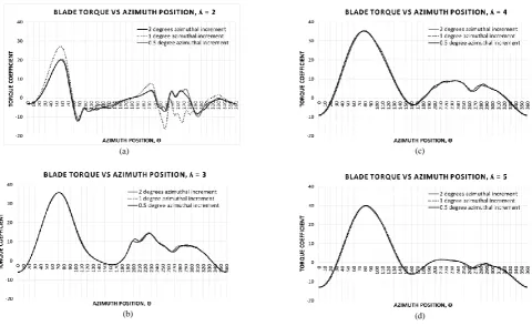
To capture the accurate unsteady physics for the simulation of the flow field, sufficient temporal resolution is required. The time step size, Δt must be small enough to resolve time-dependent features, but also must be balanced on the trade-off to longer computational time. For this study, three different temporal resolutions equivalent to the specific rotational displacement at the azimuth were tested (0.5°ω-1_,

1.0°ω-1_{, and 2.0°ω}-1_{) for four different values of tip speed}

ratio (λ = 2, 3, 4 and 5). The number of iterations per time step was set to 50 and the turbines were run to minimum of 10 full rotations.

It was observed that there was little difference among the studied time step sizes across different λ. In fact, the variance just ranges from 1.86 x 10-6 _{to 7.61 x 10}-7_{. The study}

(a)

(b)

(c)

(d)

Fig. 5. Result of simulation on torque coefficient values for different time step size at (a) λ=2, (b) λ=3, (c) λ=4, and (d) λ=5

Meanwhile the highest coefficient of performance, Cp, was found to be at λ = 4 with a value of 0.29. This result is consistent with published literature where the maximum coefficient of performance for a Darrieus vertical axis wind turbine is at the tip speed ratio of 4. The Cp for λ = 2 is observed to be practically zero while those of λ = 3 and 5 are about 0.23 and 0.13, respectively.

Fig. 6. Power Coefficient curve at different tip speed ratios, Δt = 2°.

G. Simulation Phases

The tip speed ratio of 4 was chosen primarily due to the result obtained where the maximum power coefficient, Cp, was found and agrees with the previously established literatures and studies. It was also found out that there was no significant variance among the three time-step size studied. Therefore, the 2.0 degrees was chosen to save time for the simulation.

The second phase of the study involves the simulation of different turbine distances arranged in triangular configuration (Figure 7). The upwind rotor is denoted as

is denoted as turbine 2. The downwind rotor next to the upper boundary is denoted as turbine 3. Twelve, eight and four equivalent rotor diameter distances angled at 60 degrees to each other were simulated and the average Cp of the cluster calculated from standard definition. The different turbine arrangements were subjected to a steady wind flow of 5 m/s reckoned from the inlet section of the computational domain. All the other simulation settings adopted the best values from the preceding study on mesh settings, turbulence model, convergence criteria, and time step study.

III. RESULTSANDDISCUSSION

In this study, the performance of three turbines arranged in triangular-shaped cluster fixed at oblique angles of 60 degrees with varying distances were simulated. Coefficient of performance was computed for the cluster and compared to the coefficient of performance obtained for an isolated turbine. The computational domain for the distance study can be found in Figure 7.

Fig 7. Computational Domain for Turbine Distance Study Table 1. Results for three co-rotating turbines at 12 rotor distance spacing.

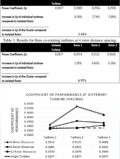
Table 2. Results for three co-rotating turbines at 8 rotor distance spacing.

Table 3. Results for three co-rotating turbines at 4 rotor distance spacing.

Fig. 8. Summary of Coefficient of Performance Computed across different turbine spacing. For comparison, the coefficient of performance for a single

turbine is plotted as the black dashed line.

At 8 rotor distances, the turbine cluster performance improved by 1.64% compared to isolated turbines (Table 2). Rotor 1, which is the upstream rotor didn’t improve significantly (+0.28%) while the two turbines at the back have improvement of 2.74% and 2.00% for the left and right turbines, respectively.

Significant improvement was observed for cluster containing turbines with 4 rotor diameter spacing (Table 3). There was an increase of 4.97% for the turbine cluster and the individual turbine performance were also seen to have increased significantly at 8.45% and 5.18% for turbine 2 and 3. The performance of turbine 1 (the upwind turbine) did not increase significantly as expected (+1.28%).

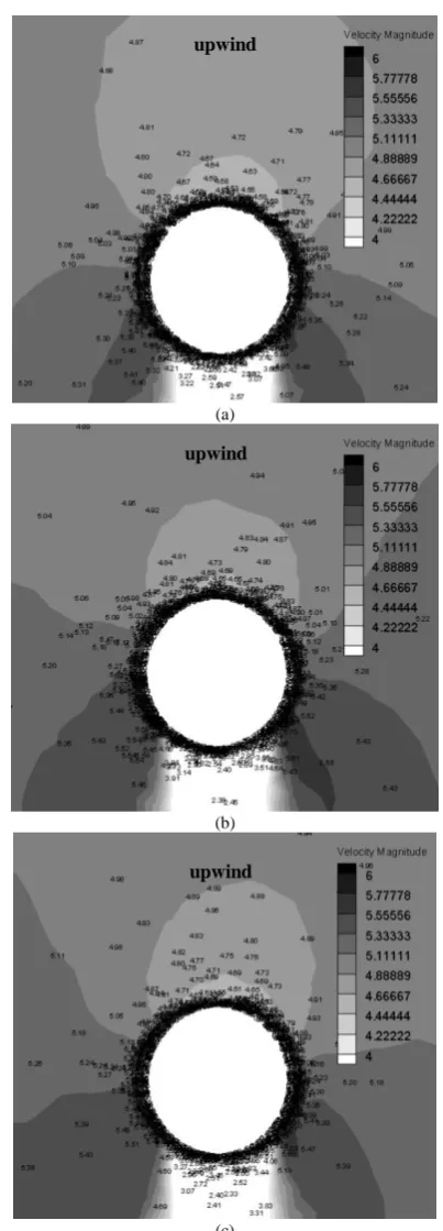
For the 4 rotor distance spacing, it is apparent that turbine number 2 exhibits the highest torque coefficient compared to the other turbines. With the same angular speed, it is conclusive that turbine 2 give the highest performance among the 3 turbines. The characteristic of the incoming wind as seen by the individual turbines can be explored to further explain the increased performance of the cluster. The velocity mapping around the turbines in Figure 10 show increased values of velocities going to the downwind turbines.

A closer look of the velocity values around the turbines will give us the impression that incoming wind stream to turbines 2 and 3 were faster compared to turbine 1, especially the area in front of the respective turbines and the oblique region between turbine 1 and 2, and turbine 1 and 3. The increase in the incoming velocity, especially in the oblique region between the upwind and downwind turbines can be described by the funnel effect. Incoming wind stream at fixed speed from the inlet boundary passes through a relatively narrow region i.e. restriction and “squeezes” in- between the turbines resulting in increased speed. As the distance between the turbines increases, the effect of restriction declines and at 12 rotor distances, the increase in the performance of individual turbines is undetectable.

To investigate the incoming wind stream velocity to the respective turbines, a velocity monitor was placed in front of each turbines one half equivalent turbine diameter away from the airfoils. It was found out that the average velocity as seen by each turbine at that particular distance in front of them are 4.641 m/s, 4.742 m/s and 4.707 m/s for turbines 1, 2 and 3, respectively compared to 4.622 m/s in the single, isolated turbine. Higher local wind speeds affect the generated forces on the rotor blades leading to the improvement in cluster performance. The computed Cp improvements are +1.28%, 8.45% and +5.18% for turbines 1, 2 and 3, respectively.

Fig 9. Torque Coefficient for one blade at 4 rotor distance configuration.

(a)

(b)

Figure 10 shows the contour plot of the velocity magnitude within the vicinity of the rotors. Overlayed are the nodal values for more detailed inspection. As one can see, the contours with slightly higher magnitudes surround the downwind rotors more than turbine 1. Values exceeding 5m/s are slightly more upwind (top of each image for Figures 10b and 10c) suggesting higher local wind velocities within the streamlines that pass through the rotor blade path. The contour bands with velocities lower than 5m/s can be seen to be wider in front of turbine 1 (Figure 10a).

IV. SUMMARY AND CONCLUSION

An array of three turbines arranged in triangular position with oblique angles of 60o _{were simulated at different}

equivalent rotor diameters. The results showed that at the distance of 12 equivalent rotor diameters, the effect of restriction to wind flow resulting to increased wind speed diminished and the individual turbine performance is essentially the same to the performance of an isolated turbine. Meanwhile at 4 equivalent rotor distance, the observed wind speed one half rotor diameter away from the turbines increased compared to single, isolated turbine resulting to almost proportionate increased in performance.

REFERENCES

[1] Sanderse, B., “Aerodynamics of Wind Turbine Wakes: Literature Review”, Energy Research Center of the Netherlands

[2] Neustadter, H.E., Spera, D.A., 1985, “Method for evaluating the wind turbine wake effects on wind farm performance”.

[3] Danao, L.,Bausas, M., 2015, “The Aerodynamics of a camber-bladed vertical axis wind turbine in unsteady wind”, MS Thesis, University of the Philippines Diliman

[4] Shaheen, M., Abdallah, S., 2015, “Development of efficient vertical axis wind turbine clustered farms”, Renewable and Sustainable Energy Reviews 63 (2016) 237-244

[5] Hezavah, D., et al, 2016, “Cluster Design for Vertical Axis Wind Turbine Farms”, Princeton University

[6] Sanderse, B., “Aerodynamics of Wind Turbine Wakes: Literature Review”, energy Research Center of the Netherlands

[7] Bons, N., “Optimization of Vertical Axis Wind Turbine Farm Layout”, American Institute of Aeronautics and Astronautics

[8] M.C. Claessnes, 2006, “Master’s Thesis: The Design and Testing of Airfoils for Application in Small Vertical Axis Wind Turbines”, Delft University of Technology

[9] Sibayan, F., 2011, “National Renewable Energy Plan 2011”, Philippine Department of Energy

[10] Wekesa, M., Danao, L., et al 2014, “A Numerical Analysis of unsteady inflow wind for site specific vertical axis wind turbine: A case study for Marsabit and Garissa in Kenya”, Elsevier Journal. [11] M.O.L. Hansen, 2008, “Aerodynamics of wind turbine, 2nd Ed.”,

Earthscan London

[12] M.M. Salim, et al , 2009, “Wall y+ Strategy for Dealing with Wall-bounded Turbulent Flow.”, Proceedings of the International Multiconference of Engineers and Computer Scientist, Vol II”, [13] Gridgen User Manual version 15

[14] Kathik, TSD, 2009, “Turbulence Models and their Applications”, 10th Indo German Winter Academy, Department of Mechanical Engineering, IIT Madras.

[15] www.engineering.com – Choosing the Right Turbulence Model for Your CFD Simulation.

[16] Raciti Castelli M, Englaro A, Benini E, 2011, “The Darrieus wind turbine: proposal for a new performance prediction model based on Cfd”

[17] Bardina J.E., Huang P.G., Coakley, T.J., 1997, “Turbulence Modeling and Validation, Testing, and Development”, Ames Research Center,

upwind

upwind