Abstract—A Strategy for modelling rotating annular flow within CFD is developed with the aid of the wall y+. The strategy will allow the pressure loss, and the effect any drilling tools has on this, to be investigated and analyzed at a reduced time and cost compared to more conventional methods. Five turbulence models were investigated and the k – ω model was found to be the most accurate for a wall y+ of less than 5 due to the low Reynolds number found in these flow situations. The k – ε model performed least well, upon investigation of the turbulence models it was found that there was a direct link between the turbulent intensity found in the annulus and the performance in predicting pressure loss. The k – ε model was found to drastically over predict the turbulent kinetic energy for the mesh set up and thus gave inaccurate results regarding the pressure loss in the annulus. This paper suggests that a structured mesh with a y+ < 5 and the k – ω turbulence model will provide sufficiently accurate data in the investigation of pressure loss in an annulus.
Index Terms— Annular Flow, CFD, Drilling, Rotating, Wall Y+
I. INTRODUCTION
URING he current climate in the oil & gas industry, innovation and efficiency are needed more than ever to reduce costs. An area where time and money could be significantly saved is during the development of drilling tools. While tools are intended to enhance drilling efficiency, the negative impact they have must also be understood during the development stage of the product. Maintaining downhole pressure to within the required window is currently a major challenge for drilling engineers, especially in horizontal and extended reach (ERD) wells [1]. It is, therefore, vital that the effect the drilling tool will have on the pressure loss within the annuals is known during the development stage of the product, so that its performance in actual drilling operations is better understood. This can be done through creating a prototype of the intended product and testing it through an experimental set-up, however, this can be costly and time-consuming. Computational Fluid Dynamics (CFD) is a method to overcome this problem by numerically modelling the product and its effect on the flow
Manuscript received December 1, 2017.
Participation at the conference was supported in part by the Institution of Mechanical Engineers (IMechE) and the Mechanical Engineering Class Grant at the University of Dundee.
Andrew A. Davidson was a student at the University of Dundee, UK. He is now a graduate engineer at Omexom, Perth, UK. (email: [email protected])
Salim M. Salim is with the University of Dundee, DD1 4HN, UK. (phone: 44-01382381378; e-mail: [email protected] ).
.
properties.
This paper will develop a strategy for modelling rotating annular flow of drilling fluid to investigate the pressure loss in an annulus, the strategy can then be transferred to incorporate the desired drilling tool. This creates huge benefits to companies who cannot afford the time or cost in producing physical prototypes of potential designs. By computational modelling the design and its impact on the fluid properties, the need for a physical prototype can be removed until the very final stages of product development.
This will be achieved by replicating experimental data in ANSYS FLUENT and investigating five turbulence models available within the software. A strategy will then be established with the aid of the wall y+ value to investigate the most suitable turbulence model and mesh configuration in FLUENT. The most time-consuming section of a CFD study can be generating a suitable mesh [2]. The most conventional method, known as a grid independence test, is to run many simulations with different mesh sizes and configurations until the results match experimental data. This removes one of the main advantages of CFD compared to experiments by increasing the time taken to complete a numerical simulation. The y+ can be used as guidance for developing a reliable mesh and turbulence model strategy thus removing the need and time for a grid independence test.
The wall y+is a non- dimensional number which indicates which section of the turbulent boundary layer, caused by the wall that the mesh resolves. It is defined in (1) and is covered in detail by Salim and Cheah [3]:
(1)
II. BACKGROUND
A. Previous Work on Wall Y+
Salim and Cheah [3] investigated a strategy for dealing with 2D wall bounded turbulent flows using the wall y+ as guidance for mesh configuration and the most suitable turbulence model. The main applications for this are situations where reliable experimental data is not available to validate a CFD model. The investigation found that a wall
y+ value in the range of 30 – 60 provides acceptable results. They also suggest the mesh should not be within the buffer region as neither the near wall treatments or wall function can solve it accurately and thus the overall solution is inaccurate. This paper shows the effectiveness of using the
y+ as a tool to assist in creating a suitable mesh and turbulence model combination. Ariff et al. [4] developed on
Wall Y
+
Strategy for Modelling Rotating
Annular Flow Using CFD
Andrew A. Davidson, and Salim M. Salim,
CEng, MIMechE, Member, IAENG
this work and carried out an investigation to deal with 3-D turbulent flows over a cube by using the y+as guidance. The work on wall y+ from both these papers will serve as guidance for this paper as both papers clearly indicate the effectiveness of the y+ as a tool for developing a reliable meshing strategy. By having a clear mesh and turbulence model strategy, the need for physical validation can be removed for flow scenarios where experimental data is difficult of complex to retrieve. This in turn will allow tool designers to assess the effectiveness of their tool, and any potential issues with it, before a prototype is made.
B. Effectiveness of CFD in the Oil & Gas Industry
CFD is used within many industries to make improvements or provide greater analysis that would be impossible to achieve by other means, and the oil & gas industry is no different. CFD is widely used for a number of key areas such as flow assurance and the investigation of cuttings transport [5, 6, 7]. While CFD is undoubtable being applied for the development of drilling tools, this paper is focusing on creating a strategy that provides validation for flow scenarios where experimental data difficult or not possible to obtain.
These papers prove the effectiveness of CFD to investigate various parameters found during drilling operations. One of the reasons CFD may not be implemented is due to the time taken to set up a numerical study and the ability to validate it. There is therefore a need for a fast, reliable modelling strategy to allow efficient analysis of drilling tools.
III. METHODOLOGY
A. Experimental Set – up
The CFD model was validated by the experiment conducted by McCann et al. [8]. The drilling fluid enters the annulus at the mud inlet, where the required flow rate is achieved using pumps. The annulus is made up of a 31.75 mm diameter stainless steel shaft to replicate the drillpipe. The wellbore is represented by an acrylic tube of 38.1mm diameter. The set up allows for the annulus to be concentric or fully eccentric while the motor can produce rotation speeds of the drillpipe up to 900 RPM. The pressures are obtained by two pressure taps, 1.22m apart, at each end of the annulus. A variety of fluids, pipe rotation speeds and annulus alignments were tested in this paper. The focus on this project will be on increasing pipe rotation for the concentric annulus on a non-Newtonian fluid, this fluid is denoted as Fluid B in the paper. This strongly represent the conditions of drilling and will act as the most relevant to creating a useful strategy.
B. Computational Domain and Boundary Conditions
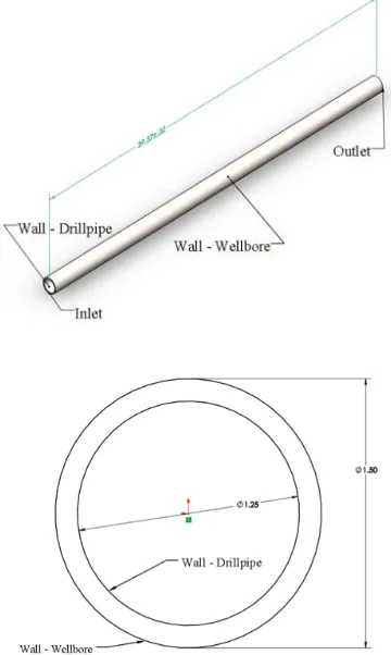
Numerical simulations are carried out using FLUENT to replicate the experimental study carried out by McCann et al. [8] where the study focuses on the effect of pressure loss due to the increasing rotation of the drillpipe. The annular space was created in ANSYS Design Modeller. A velocity Inlet and pressure Outlet are created as shown in Fig. 1. The Outerwall is stationary to represent the wellbore while the inner wall rotates as the drillpipe would. The No-Slip
[image:2.595.340.520.98.399.2]condition is applied to each was in the numerical simulation. The flow Inlet speed is 0.95 m.s-1 and the wall rotations speed range from 0-800 RPM.
Fig. 1. Computational domain generated in ANSYS for present study.
The length of the annulus is created to ensure fully developed flow. The initial flow in the pipe is known as the hydrodynamic entrance region. In this area, the flow profile is still developing and so the length of the pipe must be large enough to ensure the velocity profile is fully developed. The length was taken from the paper by Sorgun [9] the equation of fully developed flow is given in (2)
(2)
Where is the Reynolds number for a Power – Law fluid which is found through (3) defined as
(3)
C. Mesh
benchmark for the investigation.
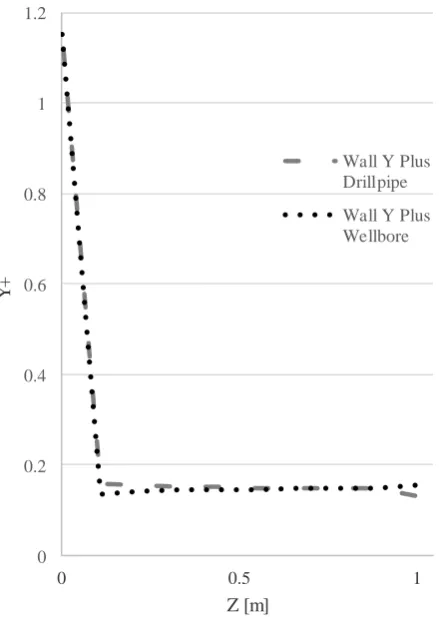
The mesh had a total of 501,000 cells. The number of cells was kept as low as possible to reduce computational times. This mesh and boundary condition combination produced a y+ value of 0.175, well below the threshold required. See Fig. 2.
0 0.2 0.4 0.6 0.8 1 1.2
0 0.5 1
Y+
Z [m]
[image:3.595.59.279.145.454.2]Wall Y Plus Drillpipe Wall Y Plus Wellbore
Fig. 2. Wall y+ for inner and outer wall.
D. Fluid properties
The fluid properties were selected to replicate the power-Law fluid used in the McCann experiment. This fluid exhibits behaviors like that of drilling fluid and is therefore suitable in predicting the pressure loss within the annulus. The details of the fluid are presented in Table 1.
IV. RESULTS
A. Comparison of turbulence models
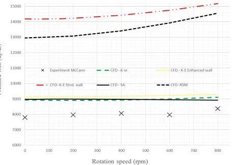
The five turbulence models within ANSYS that were investigated are standard k – ε, k – ω, k – ε Enhanced Wall, Spalart – Allmaras and RSM. All were used to replicate the experimental data by McCann, the results are displayed in Fig. 4. This provides a clear comparison of each turbulence
model in their prediction of annular pressure loss of the non – Newtonian fluid compared to the experimental data, for a
y+ value of less than 5. The pressure loss is given in Pa.meters-1 and the rotation speeds ranged from 0 to 800 RPM.
k – ω matches well with the experimental data to within 1000 Pa.m-1 and follows the trend of increasing pressure loss with increasing rotation speed. The difference between k – ω
and the experimental data is around 10 %, this is most likely due to the low number of cells used for this simulation. Spalart – Allmaras also predicts the pressure loss to a respectable level of accuracy as shown in Fig. 3. The standard k – ε and RSM models perform less well for this mesh set – up. This is to be expected flowing the ANSYS user guide [2] as the y+value is less than 5. The walls on each side of the annulus have a significant impact on fluid properties which is not accounted for in the k – ε model. Figure 4 displays that as the wall enhancement feature is applied to the k – ε model the results improve considerably to similar values of the k – ω model, this did however increase the computational time.
The standard k – ε and k – ω were analyzed further to investigate why each performs the way it does before deciding on a final strategy.
B. Analysis of k – ε and k – ω
To analyze the performance of the two turbulence models the areas that affect the pressure loss are investigated. Pressure loss is caused by the dynamic movement of the fluid. This is influenced by the velocity of the fluid and the secondary flow that is created due to the rotation of the drillpipe. The turbulence intensity and velocity profiles for each model are compared to show exactly why the k – ω
model performs the most effectively and why the k – ε model over predicts the pressure loss in the annulus.
Table 2 shows a relation in the turbulence intensity and the accuracy of the model for predicating the pressure loss.
TABLE2 TURBULENCE INTENSITY
Turbulence Model Turbulence Intensity
k – ω 2.74 %
k – ε Enhanced Wall Treat. 6.07%
RSM 12.6%
k – ε Standard 20.17%
The turbulence Intensity found in the center of the annulus for rotation speed of 800 RPM
TABLEI FLUID PROPERTIES
Symbol Quantity Units
ρ Mud Weight 9.14 (ppg)
n K
Power – Law Index Flow – Consistency
[image:3.595.341.519.554.629.2]Fig. 3. Turbulence models vs. experimental data.
The models that perform worst are found to have the highest turbulence intensity while the lower intensity corresponds to the most accurate models. The k – ω model produced a turbulence intensity of 2.7 % for a rotation speed of 800 RPM while the k – ε model produced an intensity of more than 7 times that at 20.17 %.
Due to the obvious impact of turbulence intensity on the predication of pressure loss the factors that dictate the turbulence intensity were investigated further for the maximum rotation speed. Turbulence intensity is shown in equation 4.
(4)
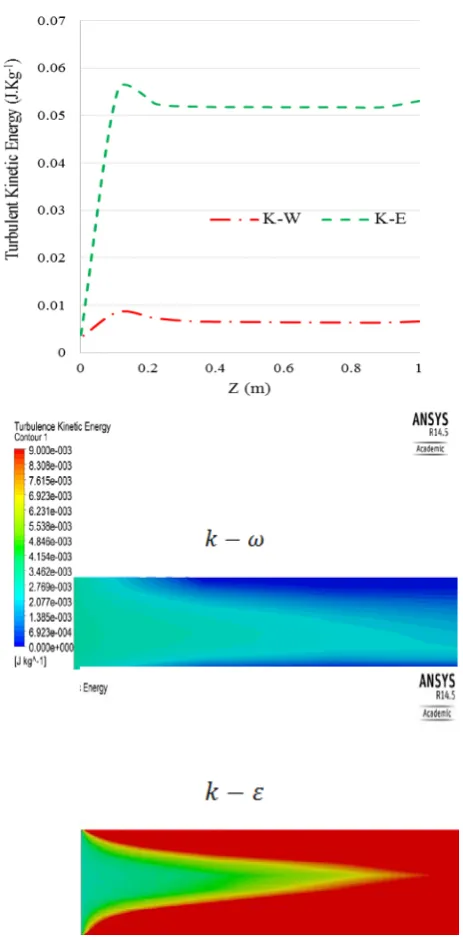
Each model predicted similar average velocity throughout differing points in the annulus. From equation 4 the factor effecting the turbulent intensity must therefore be the turbulence velocity fluctuations. The turbulence velocity fluctuations, u’, are dependent of the turbulent kinetic energy, k.
(5)
As shown in equation 5 velocity fluctuations are the square root of two thirds of the kinetic energy, k. The turbulent kinetic energy for both models were retrieved for the same location in the annular space at rotation speeds of 800 RPM for both models.
Fig. 4 displays that the k – ε turbulence model predicts a larger turbulent kinetic energy compared to the k – ω model and as a result gives an over predication of the annular pressure loss. As can been see at the entrance to the annular space, the k – ω model predicts zero kinetic energy at the walls of the annular space.in comparison the k – ε model gives a value of 9.0 x 10⁻³ J kg-1 at the walls of the annular space and throughout the annuals as the flow develops.
As both models predicted similar velocities for the drilling fluid, it can be determined that the biggest factor in the difference of results between the two models is in the predication of the turbulent kinetic energy. By over predicating the turbulent intensity the, the k – ε model predicts a greater amount of dynamic movement in the fluid giving a larger frictional pressure loss.
As previously stated the frictional pressure loss occurs due to the dynamic movement of the fluid. This is caused by the mean flow of the fluid and the secondary flow created by the rotation of the drillpipe. The velocity profiles provide evidence that the mean velocity for the two turbulence models were almost identical and therefore was not the cause of the over predication of pressure loss in the k – ε
model was compared and verified that the k – ε model predicted a higher turbulent kinetic energy and thus a higher turbulent velocity fluctuations giving a larger turbulent intensity and an over predication of the annular pressure loss.
Fig. 4. Kinetic energy at entrance to annulus for both models.
V. PROPOSED STRATEGY
The results and analysis from this flow situation determine that the k – ω turbulence model with a y+ of less than 5 would be the most suitable combination for obtaining annular pressure loss values within a rotating annulus for non – Newtonian fluids. This is summarized in Table 3.
VI. CONCLUSION
This study has displayed the use of the wall y+ as an effective tool in selecting the most suitable turbulence model and mesh configuration for predicting the pressure loss in a rotating annulus. Based on previous work by Salim and
Cheah [3], this project utilizes the wall y+ value as a method for creating a reliable meshing strategy for rotating annular flow in the oil & gas industry. The analysis of the turbulence models within ANSYS FLUENT has allowed a strategy to be recommended for predicting the pressure loss in a faster and more cost-effective manner than if it was to be found through experimental means. This report suggests a highly structured mesh with a y+ vale of less than 5 and the k – ω turbulence model. Due to the difficulties drilling engineers face with ECD management, especially in ERD wells, it is vital that the positive or negative impact tools have on this are known. The use of this strategy will allow designers of drilling tools to gain an understanding of how their tool will impact the pressure loss in an annulus during the development stage thus reducing the cost of expensive prototypes and experimental testing before the final design is created.
REFERENCES
[1] S. Zharkeshov, , "Combatting ECD challenges," Oilfield Technology, pp. 29-34, September 2016.
[2] C. E. Baukal Jr., Computational Fluid Dynamics in Industrial Combustion, p. 547.
[3] S. M. Salim and S. C. Cheah, "Wall y+ Strategy for Dealing with Wall-bounded Turbulent Flows," 2009.
[4] M. ARIFF, S. M. SALIM and S. Cheong CHEAH, "WALL Y+ APPROACH FOR DEALING WITH TURBULENT FLOW OVER A SURFACE MOUNTED CUBE: PART 1 – LOW REYNOLDS NUMBER".
[5] T. N. Ofei and W. Pao, CFD Method for Predicting Annular Pressure Losses and Cuttings Concentration in Eccentric Horizontal Wells.
[6] O. Erge, E. Ozbayoglu, S. Z.Miska, M. Yu and N. Takach, "EquivalentcirculatingdensitymodelingofYieldPowerLaw fluids validatedwithCFDapproach," 2015.
[7] M. Sorgun and E. Ulker, Modeling and Experimental Study of Solid–Liquid Two-Phase Pressure Drop in Horizontal Wellbores With Pipe Rotation, 2016.
[8] R. McCann and M. Quigley, "Effects of High-Speed Pipe Rotation on Pressures in Narrow Anuli," 1995.
[9] M. SORGUN, J. J. SCHUBERT, M. E. OZBAYOGLU and I. AYDIN, MODELING OF NEWTONIAN FLUIDS IN ANNULAR GEOMETRIES WITH INNER PIPE ROTATION.
[10] ANSYS, ANSYS Fluent 12.0 User Guide. TABLE3 PROPOSED STRATEGY
Turbulence Model y+
k – ω <5
[image:5.595.335.510.299.349.2]