A Compact Difference Scheme for One-dimensional Nonlinear Delay Reaction-diffusion Equations with Variable Coefﬁcient

(1)

A Compact Difference Scheme for

One-dimensional Nonlinear Delay

Reaction-diffusion Equations with Variable

Coefficient

Jianqiang Xie, Dingwen Deng

∗

_{, and Huasheng Zheng}

Abstract—First of all, a compact difference scheme (CDS) is established for one-dimensional (1D) nonlinear reaction-diffusion equations (RDEs) with a fixed delay. By the energy method, it is proved that the difference solution converges to exact solution with a convergence order of O(τ2₊_h4₎ _in L∞₋_{norm. Then, a Richardson extrapolation method (REM)}

is applied to make the final solution fourth-order accurate in both time and space. Besides, the extensions of the solver to other complex delay problems are studied in detail. Finally, numerical results demonstrate the high accuracy and efficiency of our algorithms.

Index Terms—Delay reaction-diffusion equations; Compact difference scheme; Convergence;

I. INTRODUCTION

Delay partial differential equations have been widely ap-plied in economics, physics, ecology, medicine, engineering control, climate model, computer-aided design and many other fields of science (cf. [1]–[6]). However, it is impossible to get their analytical solutions. Hence, it is very significant to develop high-performance numerical algorithms for this kind of equations.

In this paper, we use the CDS (cf. [2]–[4], [7]–[12]) to solve the initial boundary value problems (IBVPs) as follows:

∂u ∂t −

∂ ∂x

µ

a(x)∂u

∂x

¶

=f(u(x, t), u(x, t−s), x, t),

(x, t)∈Ω×(0, T], (1a)

u(x, t) =ϕ(x, t), (x, t)∈Ω×[−s,0], (1b)

u(a, t) =α(t), u(b, t) =β(t), t∈(0, T], (1c) where Ω := [a, b] and s > 0 is a constant fixed delay. Sufficiently smooth function a(x) fulfills the boundedness, i.e. ∃ c11, c22 > 0, such that, c11 ≤ a(x) ≤ c22.

Also, we suppose that function f(u(x, t), u(x, t−s), x, t)

is sufficiently smooth, and satisfies

|f(µ+ε1, υ+ε2, x, t)−f(µ, υ, x, t)| ≤c1|ε1|+c2|ε2|, (2) This work is partially supported by the National Natural Science Foundation of China (Grant Nos. 11401294, 11326046), Youth Nat-ural Science Foundation of Jiangxi Provincial Education Department (Grant No. GJJ14545), China Postdoctoral Science Foundation (Grant No. 2015M582631) and State Scholarship Fund of CSC for Overseas Studies (NO. 201608360086).

Jianqiang Xie, Dingwen Deng and Huasheng Zheng are with the College of Mathematics and Information Science, Nanchang Hangkong University, Nanchang 330063, China

Also, Dingwen Deng is with the School of Mathematics and Statistics, Xi’an Jiaotong University, Xi’an 710049, China. He is the corresponding author. (e-mail: [email protected])

in which ε1, ε2 are arbitrary real numbers, c1 and c2 are

positive constants.

Many numerical methods including finite difference meth-ods (cf. [2], [3]), local discontinuous Galerkin methmeth-ods (cf. [5]), have been successfully developed for solving IBVPs (1a)–(1c) with a(x) = 1. However, as we know, little attention has been paid on numerical solutions of IBVPs (1a)–(1c). This study aims at making up for this work.

II. CONSTRUCTION OF COMPACT DIFFERENCE SCHEME This section concentrates on the derivation of the CDS for problems (1a)–(1c).

A. Partition and Notations

Leth= (b−a)/M (M ∈Z+₎ _{be spatial mesh size. For}

temporal discretization, constrained temporal grid, namely,

τ =s/n (n∈Z+₎_{, is used. Setting}_x

i =a+ih,tk =kτ, the domain Ω ×(0, T] is covered by Ωh × Ωτ, where

Ωh = {xi|0 ≤ i ≤ M} and Ωτ = {tk| −n ≤ k ≤ N},

N = [T /τ]. Let {vk

i|0 ≤ i ≤ M,−n ≤ k ≤ N} be a grid function on Ωhτ. Then we introduce the fol-lowing notations: δtvik+1/2 = (vik+1 − vik)/τ, δ+tvik =

(3δtvik+1/2 − δtvki−1/2)/2, δxvik+1/2 = (vik+1 − vki)/h,

δ0xvik= (vik+1−vik−1)/2h,δx(aδxv)ki = (ai+1/2δxvki+1/2−

ai−1/2δxv_ik₋₁_/₂)/h.

B. Construction of the compact difference scheme

Let

v= ∂

∂x

µ

a(x)∂u

∂x

¶

. (3)

Define grid functions Uk

i = u(xi, tk), Vik = v(xi, tk),

0≤i≤M,−n≤k≤N. The application of second order backward differentiation formula (BDF2) to approximate (1a) at the point(xi, tk+1)gives that

δ_t+Uk

i −Vik+1=f(Uik+1, Uik+1−n, xi, tk+1) +τ2rki, (4) where

rk i =−

1 3

∂3_u

∂t3(xi, tk+1) +

τ

4

∂4_u

∂t4(xi, tk+1)

−7τ

2

60

∂5_u

∂t5(xi, ξk+1), ξk+1∈(tk, tk+1).

Using compact finite difference scheme to approximate (3) at the point(xi, tk+1)yields that

AhVik+1=δx(ˆaδxU)ki+1+O(h4), (5)

IAENG International Journal of Applied Mathematics, 47:1, IJAM_47_1_03

(2)

where the compact operatorAh (see [11]) is defined as

Ahuki+1=     

uk_i+1+h 2

12(δ 2

xuki+1−δ0x(

a0 au)

k+1

i ),

1≤i≤M−1, uk+1

i , i= 0or M, where ˜a = (a0₎2_/a₋_a00_/₂_, _ˆ_a ₌_a₋₍_h2_˜_a₎_/₁₂_, _a0 _and_a00

denote the first and second order spatial derivatives ofa(x), respectively.

MultiplyingAhto the both sides of (4), then inserting (5) into the resulting formula, we get

Ahδ+tUik−δx(ˆaδxU)ki+1=Ahf(Uik+1, Uik+1−n, xi, tk+1)

+Rk

i, 1≤i≤M−1, 0≤k≤N−1, (6) whereRk

i =O(τ2+h4), by which we can suppose that ∃

c >0, such that|Rk

i| ≤c(τ2+h4). Omitting the small term Rk

i and then replacingUik with its approximations uk

i in (6), a CDS is devised as follows

Ahδt+uki −δx(ˆaδxu)ki+1=Ahf(uki+1, uik+1−n, xi, tk+1),

1≤i≤M −1, 0≤k≤N−1, (7)

uk0=α(tk), ukM =β(tk), 1≤k≤N, (8)

uki =ϕ(xi, tk), 0≤i≤M, −n≤k≤0. (9) At each time level, the CDS (7)–(9) is a linear tridiagonal system with strictly diagonally dominant coefficient matrix, thus it has an unique solution.

III. ANALYSIS OF THE COMPACT DIFFERENCE SCHEME In this section, we study the convergence of CDS (7)–(9). Firstly, we further assume that ∃ positive constants c3, c4

such that|a0_/a_{| ≤}_c

4,|(a0/a) 0

| ≤c4,c3≤ˆa≤c4.

Let V ={v|v = (v0, v1,· · · , vM), v0 = vM = 0} be a grid function space on Ωh.∀ v,w∈V, we define the inner products and discrete norms as follows(v, w) =hMP−1

i=1

viwi,

kvk2_{= (}_{v, v}₎_,_k_v_k

∞= max

0≤i≤M|vi|,|v|

2

1=h

M_P−1

i=0

(δxvi+1 2)

2_,

|v|2 1∗=h

M_P−1

i=0 ˆ

a_i₊1

2(δxvi+12)

2_.

By the definition of |v|1∗, it is easy to get the lemma 1.

Lemma 1 ∀v∈V, we have √c3|v|1≤ |v|1∗≤√c4|v|1. Lemma 2(cf. [2]) ∀ v∈V, we obtain

kvk∞≤(

√

b−a|v|1)/2, kvk ≤[(b−a)|v|1]/√6.

Lemma 3 ∀v∈V, it holds that

(2

3 −

c4h2 24 )kvk

2_≤₍_A

hv, v)≤(1 + c4h

2

24 )kvk 2_.

Proof. Noting Ahvi = vi + h 2

12(δx2vi −δ0x(a

0

av)i), and utilizing the discrete Green formula yield that

(Ahv, v) =kvk2−h

2

12kδxvk 2

−h

2

12h

M_X−1

i=1 (a0

a)i+1−(a

0

a)i

2h vi+1vi. (10)

The use ofkδxvk2≤4h−2kvk2to (10) deduces the claimed result.

Theorem 1 Let u(x, t) ∈ Cx,t6,3(Ω×(0, T]) be the exact solution of (1a)–(1c),uk _{be the solution of the scheme (7)–} (9) at the time levelk, respectively. Denoteek

i =u(xi, tk)−

uk

i, 0 ≤ i ≤ M, −n ≤ k ≤ N. Then, as h and τ are sufficiently small, we conclude that

kekk∞≤C(τ2+h4), 0≤k≤N, (11)

where

C=(b−a)

2 c

r

3T c3 exp

µ

13T(b−a)2 12c3 max(c

2 1, c22)

¶

.

Proof. Denote Gk_i+1 = f(U_ik+1, U_ik+1−n, xi, tk+1) −

f(uk_i+1, u_ik+1−n, xi, tk+1). Subtracting (7) from (6), the er-ror equations are derived as follows:

Ahδ+teki −δx(ˆaδxe)ki+1=AhGki+1+Rki,

1≤i≤M−1, 0≤k≤N−1, (12)

ek0= 0, ekM = 0, 1≤k≤N, (13)

ek

i = 0, 0≤i≤M, −n≤k≤0. (14) In the following, mathematical induction is applied to prove this theorem. From (14), it follows that kek_k

∞ = 0,−n≤ k≤0. Assuming that (11) is valid for 0≤k ≤l, we will prove that it is also true fork=l+ 1.

Using inequality−ab≥ −(a2₊_b2₎_/₂ _{gives that}

h

M_X−1

i=1

(Ahδt+eki)δtek+ 1 2 i

≥h

M_X−1

i=1

(Ahδtek+ 1 2 i )δtek+

1 2 i + 1 4 © h

M_X−1

i=1

1 2 i

−h

M_X−1

i=1

(Ahδtek− 1 2 i )δtek−

1 2 i

ª

. (15)

From the discrete Green formula and inequalitya(a−b)≥

(a2₋_b2₎_/₂_{, it follows that}

−h

M_X−1

i=1

(δx(ˆaδxe)ik+1)δtek+ 1 2 i ≥

(|ek+1_|2

1∗− |ek|21∗)

2τ . (16)

Next, we estimate

h

M_X−1

i=1

(AhGki+1)δtek+ 1 2 i

≤h

M_X−1

i=1

¡

Ah(c1|eki+1|+c2|eki+1−n|) ¢

|δtek+ 1 2 i |

:=A1+A2+A3+A4+A5. (17)

Applyingab≤a2_/₍₂_ε_{) + (}_εb2₎_/₂_{, we arrive at}

A1=

h

12

M_X−1

i=1

(c1|eki+1+1|+c2|eki+1+1−n|)|δtek+ 1 2 i |

≤(c

2

1kek+1k2+c22kek+1−nk2)

12ε +

ε

24kδte

k+1

2k2, (18)

A2= 5h

6

M_X−1

i=1

(c1|eki+1|+c2|eki+1−n|)|δtek+ 1 2 i |

≤5(c

2

6ε +

5ε

12kδte

k+1

2k2, (19)

IAENG International Journal of Applied Mathematics, 47:1, IJAM_47_1_03

(3)

A3= h 12

M_X−1

i=1

(c1|eki−+11|+c2|eki−+11−n|)|δtek+ 1 2 i |

≤ (c

2

12ε +

ε

24kδte

k+1

2k2, (20)

A4= h 24

M_X−1

i=1

(c1|eki−+11|+c2|eki−+11−n|)h(

a0

a)i−1|δte

k+1 2 i |

≤(c

2

24ε +

c2 4h2ε

48 kδte

k+1

2k2, (21)

A5=−h 24

M_X−1

i=1

(c1|eki+1+1|+c2|eki+1+1−n|)h(

a0

a)i+1|δte

k+1 2 i |

≤(c21kek+1k2+c22kek+1−nk2)

24ε +

c2 4h2ε

48 kδte

k+1

2k2. (22) The substitution of (18)–(22) into (17) yields that

h

M_X−1

i=1

(AhGki+1)δtek+ 1 2 i ≤

13(c2

1kek+1k2+c22kek+1−nk2) 12ε

+ε 2kδte

k+1 2k2+c

2 4h2ε

24 kδte

k+1

2k2. (23)

Besides, usingε-inequality obtains that

h

M_X−1

i=1

Rkiδtek+ 1 2 i ≤

1 2εkR

k_k2₊ε 2kδte

k+1

2k2. (24) Multiplying (12) by hδtek+

1 2

i , summing ifrom1 toM−1, and then substituting (15), (16), (23), (24) into the resulting equation, we have

(|ek+1_|2

1∗− |ek|21∗)

2τ +h

M_X−1

i=1

1 2 i + 1 4 © h

M_X−1

i=1

1 2 i −h

M_X−1

i=1

(Ahδtek− 1 2 i )δtek−

1 2 i

ª

≤ 13(c

2

12ε +

ε

24c 2

4h2kδtek+ 1 2k2

+ 1

2εkR

k_k2₊_ε_k_δ

tek+ 1

2k2. (25)

Multiplying 2τ to the both sides of (25), summing k from

0 tol, using Lemma 2 and Lemma3, and then lettingε= [2/3−(c4h2)/24]/[1 + (c24h2)/24], we arrive at

|el+1|21∗≤3(b−a)c2T(τ2+h4)2

+13τ 6 (b−a)

2_max(_c2 1, c22)

l X

k=1

|ek_|2

1, (26)

in whichhis taken to makeε≥1/3becausehis sufficiently small. The applications of lemma1and the discrete Gronwall inequality to (26) yield

|el+1_|2

1≤

3

c3

(b−a)c2_T₍_τ2₊_h4₎2 exp

µ

13T(b−a)2 6c3 max(c

2 1, c22)

¶

. (27)

Applying Lemma 2infers that

kel+1_k

∞≤

√

b−a

2 |e

l+1_|

1≤C(τ2+h4). (28)

By inductive principle, (11) is valid.

IV. EXTENSION TO REACTION-DIFFUSION EQUATIONS WITH SEVERAL DELAYS

This section focuses on the extensions of the CDS (7)–(9) and corresponding analytical results to the equations with several delays as follows:

             ∂u ∂t − ∂ ∂x µ

a(x)∂u

∂x

¶

=f(u(x, t), u(x, t−s1), u(x, t−s2), . . . , u(x, t−sK), x, t),(x, t)∈Ω×(0, T],

u(a, t) =α(t), u(b, t) =β(t), t∈(0, T], u(x, t) =ϕ(x, t), (x, t)∈Ω×[−˜s,0],

(29) wheres˜κ >0 (κ= 1,2, . . . , K), and s˜= max

1≤κ≤Ksκ, 0 ≤

c11 ≤ a(x) ≤c22. To preserve high-order accuracy of the

algorithms, we should utilize the constrained time integrator:

τ =s1/n1 =s2/n2=· · ·=sK/nK (κ= 1,2, . . . , K), to maket=Lsκ (L∈Z+)locate the temporal grid nodes.

In this case, CDS (7)–(9) for (1a)–(1c) can be eas-ily adapted to the numerical solution of IBVP (29) by replacing f(U_ik+1, U_ik+1−n, xi, tk+1) with f(Uik+1,

Uk+1−n1

i , Uik+1−n2, . . . , Uik+1−nK, xi, tk+1)in (7). More-over, corresponding theoretical results are derived by using the analytical methods similar to that of the solver CDS (7)– (9) as long asf(u(x, t), u(x, t−s1), u(x, t−s2), . . . , u(x, t−

sK), x, t)satisfies Lipschitz condition with respect to its 1st, 2nd, . . . ,K+ 1−th variables.

V. EXTENSIONS TO GENERAL NONLINEAR DELAY PARABOLIC EQUATIONS

This section aims to the numerical approximation of the following IBVPs:              ˜

r(x, t)∂u

∂t − ∂2_u

∂x2 −˜b(x, t)

∂u

∂x + ˜c(x, t)u= ˜f(u

(x, t), u(x, t−s), x, t), (x, t)∈[a, b]×(0, T], u(a, t) =α(t), u(b, t) =β(t), t∈(0, T], u(x, t) =ϕ(x, t), (x, t)∈[a, b]×[−s,0].

(30)

To begin with, using the skills proposed in [3], multiplying the first equation of (30) by exp¡R₀x˜b(s, t)ds¢, then IBVPs (30) is equivalently transformed into

            

r(x, t)∂u

∂t − ∂ ∂x

µ

a(x, t)∂u

∂x

¶

+c(x, t)u=f(u

(x, t), u(x, t−s), x, t), (x, t)∈[a, b]×(0, T], u(a, t) =α(t), u(b, t) =β(t), t∈(0, T], u(x, t) =ϕ(x, t), (x, t)∈[a, b]×[−s,0],

(31)

wherer(x, t) = ˜r(x, t) exp¡R₀xb˜(s, t)ds¢,a(x, t) = exp¡R₀x ˜_b₍_{s, t}₎_ds¢_,_c₍_{x, t}_{) = ˜}_c₍_{x, t}_{) exp}¡Rx

0 ˜b(s, t)ds

¢

,f(u(x, t), u(

x, t−s), x, t) = exp¡R₀x˜b(s, t)ds¢f˜(u(x, t), u(x, t−s), x, t). Analogous to (1a)–(1c), the CDS for IBVP (31) is de-signed as follows

          

Ah(rki+1δt+uik)−δx(ˆaδxu)ik+1+cki+1uki+1=Ahf(uki+1,

uk_i+1−n, xi, tk+1), 1≤i≤M −1, 0≤k≤N−1,

uk

0 =α(tk), ukM =β(tk), 1≤k≤N,

uk

i =ϕ(xi, tk), 0≤i≤M, −n≤k≤0, (32)

IAENG International Journal of Applied Mathematics, 47:1, IJAM_47_1_03

(4)

which is also adapted to solve IBVPs (31) with several delays using techniques developed in section (IV). It is easy to obtain the corresponding theoretical results similar to Theorem 1, too.

Remark Also, our CDS can be slightly modified to solve the following nonlinear parabolic equations with proportional delay [13]–[15]:

r(x, t)∂u

∂t − ∂ ∂x

µ

a(x)∂u

∂x

¶

=f(u(x, t), u(x, pt), x, t),

(33)

where (x, t) ∈ [a, b]×[0, T], 0 < p < 1. Let w(x, t) =

u(x, et₎ _for _t _≥ _t

0+ln(p), where t0 ≥ 0. Then w(x, t)

satisfies the problem: 

  

  

ˆ

r(x, t)∂w

∂t − ∂ ∂x

µ

a(x)∂w

∂x

¶

=f1(w(x, t), w(x, t−s), x, t), x∈[a, b], t∈[t0, T],

w(x, t) =u(x, et₎_, _t_∈_[₋_{s, t}_0]_,

(34)

wheres=−ln(p),rˆ(x, t) =e−t_r₍_{x, e}t₎_,_f₁₍_w₍_{x, t}₎_{, w}₍_{x, t}

−s), x, t) =f(w(x, t), w(x, t−s), x, et₎_. Therefore, wn

i is firstly obtained by using CDS (32). Then, un

i is provided by applying transformationu(x, et) =

w(x, t).

VI. NUMERICAL EXAMPLES

In this section, three numerical examples are solved to illustrate the performance of the algorithms.L∞_{-norm errors,}

which are defined by er∞(h, τ) = kekk∞, erˆ∞(h, τ) =

kˆek_k

∞, respectively, and CPU time are applied to measure

the accuracy and efficiency of the algorithms. Here, eˆk i =

u(xi, tk)−uˆki, anduˆki is computed by the following REM 





ˆ

uki =

1 21u

k

i(h, τ)−

4 7u

2k i (h,

τ

2) + 32 21u

4k i (h,

τ

4), ˆ

uk

0 =α(tk), uˆkM =β(tk).

(35)

Convergence rates in L∞_{-norm are defined as follows:} r1 = log2erer∞∞(2(h,h,τ4)τ), r2 = log2

er∞(2h,2τ)

er∞(h,τ) , r3 = log2erˆerˆ∞∞(2(h,h,τ2τ)), respectively. All computer programs are

carried out by Matlab 7.0.

Example 1 Consider the following equation with two constant delays:

∂u ∂t =

∂ ∂x

µ

a(x)∂u

∂x

¶

+ u(x, t−s1)

1 +u2₍_{x, t}₋_s₂₎+h(x, t),

where (x, t) ∈ (0,1)×(0,1], a(x) = x2_{+ 2}_, _h₍_{x, t}_{) =}

xcos(t)−2xsin(t)−[xsin(t−s1)]/[1 +x2_sin2₍_t₋_s_2)]_.

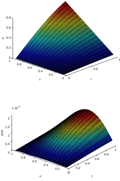
Initial-boundary conditions are determined by its exact solu-tion u(x, t) =xsin(t). The proposed solvers are applied to solve example1 withs1=s2= 0.2or s1= 0.1,s2= 0.2.

Numerical results testify the following conclusions. (1) Table I confirms that CDS (7)–(9) is second-order accurate in time and fourth-order accurate in space. Table II shows that the combination of CDS (7)–(9) with REM (35) can obtain the approximation solution of order4in both time and space.

(2) Approximation solution U and errors|eˆ|are plotted in Figure 1, from which we find that numerical oscillation does not appear, and CDS (7)–(9) combined with REM (35) has a good resolution.

0

0.5

1

0 0.2 0.4 0.6 0.8 1 0 0.2 0.4 0.6 0.8

t x

U

0 0.2

0.4 0.6

0.8 1

0 0.2 0.4 0.6 0.8 1 0 0.5 1 1.5 2

x 10−8

t x

[image:4.595.320.525.65.373.2]

error

Fig. 1. Example1withs1= 0.1, s2= 0.2(solved by the CDS (7)–(9) combined with REM (35) withh=τ= 1/20):approximation solution U (top) and error|ˆe|(bottom), respectively.

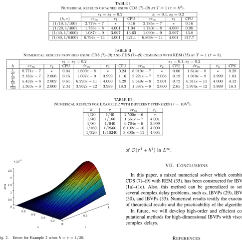
Example 2 Let Ω = [0,1]. Then, on Ω×[−0.2,1], in order to further exhibit the validity of our proposed solver, we consider the following IBVPs:

e−x∂u

∂t − ∂2_u

∂x2 −

∂u ∂x =t

2_f₍_u₍_{x, t}₎_{, u}₍_{x, t}₋₀_.₂₎_{, x, t}₎_,

where

f =−u2₍_{x, t}_{) +}_u2₍_{x, t}₋₀_._{2) +}_e−x_t−2_cos(_πx_{) +}_πt−1 sinπx+π2_t−1_cos(_πx_{) +}_t2_cos2₍_πx₎₋₍_t₋₀_.₂₎2_cos2₍_πx₎_.

Initial and boundary conditions are determined by its exact solutionu(x, t) =tcos(πx).

In view of section V, this problem can be solved using CDS (32). Table III displays the errors and convergence orders for different step-sizes. Figure 2 depicts the error surface for Example 2. From Table III and Figure 2, it is observed that numerical results are in accordance with theoretical results.

Example 3 Finally, the combination of CDS (32) with transformation w(x, t) = u(x, et₎ _{is suggested for solving} the general parabolic equation with proportional delay as follows:

t∂u ∂t −

∂ ∂x

µ

a(x)∂u

∂x

¶

=u(x, pt) +h(x, t),

wherep= 3/4,a(x) =ex_,_h₍_{x, t}_{) =}_x2_tet₋₂_ex+t₍_x₊₁₎₋

x2_ept_{. Its initial and boundary values can be determined by} the exact solutionu(x, t) =x2_et_.

IAENG International Journal of Applied Mathematics, 47:1, IJAM_47_1_03

(5)

[image:5.595.51.537.49.530.2] [image:5.595.143.451.64.133.2]

TABLE I

NUMERICAL RESULTS OBTAINED USINGCDS (7)–(9)ATT = 1(τ=h2_).

s1=s2= 0.2 s1= 0.1, s2= 0.2

(h, τ) er∞ r1 CPU er∞ r1 CPU

(1/10,1/100) 2.779e−7 ∗ 0.16 2.785e−7 ∗ 0.16 (1/20,1/400) 1.736e−8 4.001 1.04 1.740e−8 4.000 0.98 (1/40,1/1600) 1.087e−9 3.997 13.63 1.090e−9 3.997 13.8 (1/80,1/6400) 6.794e−11 4.001 321.1 6.809e−11 4.001 317.7

TABLE II

NUMERICAL RESULTS PROVIDED USINGCDS (7)–(9)ANDCDS (7)–(9)COMBINED WITHREM (35)ATT = 1(τ=h).

s1=s2= 0.2 s1= 0.1, s2= 0.2

h er∞ r2 CPU er∞ˆ r3 CPU er∞ r2 CPU er∞ˆ r3 CPU 1

20₁ 8.771e−7 ∗ 0.04 1.609e−8 ∗ 0.24 8.919e−7 ∗ 0.06 1.614e−8 ∗ 0.28 40 2.183e−7 2.006 0.15 1.007e−9 3.999 1.16 2.221e−7 2.005 0.19 1.010e−9 3.999 1.03

1

80 5.452e−8 2.002 0.61 6.293e−11 4.000 4.29 5.549e−8 2.001 0.72 6.311e−11 4.000 4.12 1

160 1.363e−8 2.000 2.34 3.962e−12 3.989 18.3 1.387e−8 2.000 2.65 3.974e−12 3.989 18.3

TABLE III

NUMERICAL RESULTS FOREXAMPLE2WITH DIFFERENT STEP-SIZES(τ= 10h2_).

h τ er∞ r1

1/20 1/40 2.500e−6 ∗ 1/40 1/160 1.561e−7 4.001 1/80 1/640 9.764e−9 3.999 1/160 1/2560 6.102e−10 4.000 1/320 1/10240 3.803e−11 4.004

0

0.5

1

0 0.2 0.4 0.6 0.8 1 0 0.5 1 1.5 2 2.5

x 10−6

t x

error

[image:5.595.53.287.554.613.2]

Fig. 2. Errors for Example 2 whenh=τ= 1/20.

TABLE IV

NUMERICAL RESULTS FOREXAMPLE3WITH DIFFERENT STEP-SIZES.

h τ er∞ r2 er∞ˆ r3 1/20 1/20 6.998e−4 ∗ 4.574e−7 ∗ 1/40 1/40 1.860e−4 1.912 2.926e−8 3.966 1/80 1/80 4.711e−5 1.981 1.832e−9 3.997 1/160 1/160 1.186e−5 1.990 1.143e−10 4.002

From Table IV and V, we can observe that the CDS (32) combined with transformationu(x, et_{) =}_w₍_{x, t}₎_{has a} convergence rate ofO(τ2₊_h4₎_in_L∞_{, and the combination}

of CDS (32), REM (35) and transformation u(x, et_{) =}

w(x, t) can provided the numerical solution with an order

TABLE V

NUMERICAL RESULTS FOREXAMPLE3 (τ=h2_).

h τ er∞ r1

1/10 1/100 3.658e−5 ∗ 1/20 1/400 2.316e−6 3.981 1/40 1/1600 1.455e−7 3.993 1/80 1/6400 9.101e−9 3.999

ofO(τ4₊_h4₎_in_L∞_.

VII. CONCLUSIONS

In this paper, a mixed numerical solver which combines CDS (7)–(9) with REM (35), has been constructed for IBVPs (1a)–(1c). Also, this method can be generalized to solve several complex delay problems, such as, IBVPs (29), IBVPs (30), and IBVPs (33). Numerical results testify the exactness of theoretical results and the practicability of the algorithms. In future, we will develop high-order and efficient com-putational methods for high-dimensional IBVPs with viscous complex delays.

REFERENCES

[1] J.Wu, “Theory and Applications of Partial Functional Differential Equations,” Springer-Verlag, New York, 1996.

[2] Z. Sun, Z. Zhang, “A linearized compact difference scheme for a class of nonlinear delay partial differential equations,” Applied Mathematical Modelling, vol. 37, pp. 742–752, 2013.

[3] Q. Zhang, C. Zhang, “A compact difference scheme combined with extrapolation techniques for solving a class of neutral delay parabolic differential equation,” Applied Mathematics Letters, vol. 26, no. 2, pp. 306–312, 2013.

[4] D. Deng, “The study of a fourth-order multistep ADI method applied to nonlinear delay reaction-diffusion equations,” Applied Numerical Mathematics, vol. 96, pp. 118–133, 2015.

[5] D. Li, C. Zhang, H. Qin, “LDG method for reaction-diffusion dynamical systems with time delay,” Applied Mathematics and Computation, vol. 217, pp. 9173–9181, 2011.

[6] Y. Guo, “Existence and exponential stability of pseudo almost periodic solutions for Mackey-Glass equation with time-varying delay,” IAENG International Journal of Applied Mathematics, vol. 46, no. 1, pp. 71-75, 2016.

[7] J. Chen and W. Chen, “Two-dimensional nonlinear wave dynamics in blasius boundary layer flow using combined compact difference methods,” IAENG International Journal of Applied Mathematics, vol. 41, no. 2, pp. 162-171, 2011.

[8] D. Deng, and T. Pan, “A fourth-order singly diagonally implicit runge-Kutta method for solving one-dimensional Burgers’ equation,” IAENG International Journal of Applied Mathematics, vol. 45, no. 4, pp. 327– 333, 2015.

IAENG International Journal of Applied Mathematics, 47:1, IJAM_47_1_03

(6)

[9] B. Wongsaijai, K. Poochinapan, and T. Disyadej, “A compact finite difference method for solving the general Rosenau-RLW equation,” IAENG International Journal of Applied Mathematics, vol. 44, no. 4, pp. 192-199, 2014.

[10] D. Deng, and J. Xie, “High-order exponential time differencing methods for solving one-dimensional Burgers’ equation,” IAENG In-ternational Journal of Computer Science, vol. 43, no. 2, pp. 167–175, 2016.

[11] Z. Sun, “An unconditionally stable andO(τ2₊_h4₎_order_L∞ con-vergence difference scheme for linear parabolic equation with variable coefficients,” Numerical Methods Partial Differential Equations, vol. 6, pp. 619–631, 2001.

[12] D. Deng, and Z. Zhang, “A new high-order algorithm for a class of nonlinear evolution equation,” Journal of Physics A: Mathematical and Theoretical 41 015202 (2008).

[13] R. Abazaria, M. Ganjib, “Extended two-dimensional DTM and its application on nonlinear PDEs with proportional delay,” International Journal of Computer Mathematics, vol. 88, no. 8, pp. 1749–1762, 2011. [14] Y. Wang, An efficient computational method for a class of singularly perturbed delay parabolic partial differential equation, International Journal of Computer Mathematics, vol. 88, no. 16, pp. 3496–3506. [15] C. Zhang, “The discrete dynamics of nonlinear

infinite-delay-differential equations,” Applied Mathematics Letters, vol. 15, no. 5, pp. 3496–3506, 2002.