A Simulation Study for Performance Validate of Indoor Location Estimation based on the Radial Weibull/Extreme-Value Weibull Distribution

A Simulation Study for Performance Validate of

Indoor Location Estimation based on the Radial

Weibull/Extreme-Value Weibull Distribution

Kosuke Okusa and Toshinari Kamakura

Abstract—We investigate the possibility of analyzing indoor location estimation under the NLoS environment by radial distribution model. In this study, we assume that the observed distance between the transmitter and receiver is a statistical radial distribution. The proposed method is based on the marginal likelihoods of radial distribution generated by positive distribution among several transmitter radio sites placed in a room. In this paper, we consider the two radial distribution model – radial Weibull distribution [9] and radial extreme value Weibull distribution [18]. To demonstrate the effectiveness of the two methods, we carried out a simulation study to assess the accuracy of the location estimation. Results indicate that high accuracy was achieved when the radial extreme value Weibull distribution based method was implemented for indoor spatial location estimation.

Index Terms—Indoor Location Estimation, Radial Distribu-tion, Extreme Value DistribuDistribu-tion, Weibull Distribution

I. INTRODUCTION

In this study, we investigated the possibility of analyzing indoor spatial location estimation under the NLoS environ-ment by radial extreme value distribution model. In recent times, the global positioning systems (GPS) are used daily to obtain locations for car navigation. These systems are very convenient, but sometimes we also require location estimation in indoor environments, for instance, to obtain nursing care information in hospitals. Indoor location estima-tion based on the GPS is very difficult because it is difficult to receive GPS signals.

A study on indoor spatial location estimation is very important in the fields of marketing science and design for public space. For instance, indoor spatial location estimation is an important tool for space planning based on the evac-uation model and shop layout planning [13], [12], [7], [6], [11] .

Recently, indoor spatial location estimation is mostly based on the received signal strength (RSS) method [8], [27], [22] , angle of arrival (AoA) method [15], [24], and time of arrival (ToA) method [23], [5], [26].

The RSS is a cost-effective method that uses general radio signals (e.g., Wi-Fi networks). However, the signal strength is affected by signal reflections and attenuation, and hence, it is not robust. Therefore, location estimation accuracy using the RSS method is very low. The AoA is a

This work was supported by JSPS KAKENHI Grant Number 30636907, 40150031.

K. Okusa is with the Department of Communication Design Science, Faculty of Design, Kyushu University, Fukuoka, 8158540 Japan, e-mail: [email protected].

T. Kamakura is with the Department of Industrial and Systems Engineer-ing, Faculty of Science and EngineerEngineer-ing, Chuo University, Tokyo, 112-8551 Japan, e-mail: [email protected].

highly accurate method that uses signal arrival directions and estimated distances. However, this method is very expensive because array signal receivers are required. The ToA method only makes use of the distance between the transmitter and the receiver. The accuracy of this method is higher than that of the RSS method and its cost is also lower than that of the AoA method. For this reason, it has been suggested that the ToA method is the most suitable method for practical indoor location estimation system [20].

In this study, we made use of the ToA data-based measure-ment system. The location estimation algorithm implemeasure-mented in previous studies were mostly based on the least-squares method. However, using the least-squares method to process the outlier value is difficult, and such data is frequently encountered in the ToA method .

To address this problem, we propose a method based on the marginal likelihoods of radial distribution generated by positive distribution among several transmitter radio sites placed within a room – radial distribution based approach [9] and radial extreme value based approach [18]. These method shows good performance for indooor location estimation, however, we still not compare the performance of two methods. In this paper, a comparison of the two methods was carried out to demonstrate its potential for practical use. To demonstrate the effectiveness of our method, we carried out a simulation study to assess the accuracy of the location estimation. The results indicate that high accuracy was achieved when the extreme distribution based method was implemented for indoor spatial location estimation.

The rest of this paper is organized as follows. In Section II, the features and problems of ToA signals are discussed. In Section III, we will present models for indoor location estimation under the NLoS environment based on the radial extreme value distribution. In Section IV, we will present some performance results from a simulation study to demon-strate the effectiveness of our model. We will conclude with a summary in Section V.

II. TIME OFARRIVAL(TOA)DATA

ToA is one of the methods used to estimate the distance between the transmitter and receiver. This method is com-puted from the travel time of radio signals between the transmitter and receiver. When the transmitter’time and the receiver’s time have been completely synchronized, the distancedbetween the transmitter and receiver is calculated as follows:

d=C(rr−rt), (1)

IAENG International Journal of Applied Mathematics, 48:2, IJAM_48_2_01

where rt andrr are transmitted and received time,

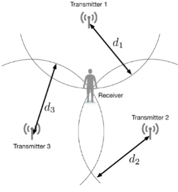
respec-tively. C is the speed of light. In an ideal circumstance, d provides accurate distance between the transmitter and receiver called the Line-of-Sight. In this case, the location of the subject is easily estimated by trilateration (Figure 1).

Fig. 1. Location estimation by trilateration (ideal case)

However, in many cases, the distancedincludes error com-ponents called Non Line-of-Sight (NLoS) [3], [25] (Figure 2).

!

"

Line-of-Sight Non Line-of-Sight

"

Fig. 2. LoS, NLoS illustration

NLoS conditions are mainly due to obstacles between the transmitter and receiver, i.e., signal reflections. In this case, the observed distancedwill be longer than the true distance. Fujita et. al.[4] reported that the observed distance of LoS and NLoS are defined as follows:

dk,LoS=

√

(x−ck1)2+ (y−ck2)2+ek (2)

dk,N LoS=

√

(x−ck1)2+ (y−ck2)2+ek+bk(3)

In the LoS case, the observed value is distributed from the true distance with error term ek ∼ N(0, σ2k), where

N(·) is the normal distribution. However, in the NLoS case, the observed value contains an additional bias term bk ∼ U(0, Bmax), where U(·) is the uniform distribution.

Bmax is the possible maximum bias value of the observed

value.

Figure 3 shows an example of the error density between the true distance and observed distance. Here, solid line represents the LoS case density, and dashed line represents the NLoS case density. Figure 3 indicates that for the NLoS case, the estimated distance is not distributed in true distance.

To address this, some studies implemented the model-based MLE approach[10], [19], [14]; however, these methods were modelized by 1-D distribution. ToA signals indicate only the distance, and not the angle. We can assume that the observed signal is a 2-D distribution and we propose the statistical radial distribution.

From the viewpoint of 2-D distribution, Kamakura & Okusa [9] proposed the radial distribution-based location estimation. However, this method did not consider the NLoS situation. For the NLoS case, Okusa & Kamakura [16], [17] proposed the NLoS bias correction approach, but this method requires iteration calculation. Therefore, it is not suitable for real-time location estimation.

In this study, we assumed that the minimum value of the observed signal is the true distance between the transmitter and receiver (Figure 5). We modeled the distribution of the minimum value (extreme value distribution) for indoor location estimation.

LoS Case

NLoS Case

Fig. 3. Error density between true distance and observed distance

III. INDOORLOCATIONESTIMATIONALGORITHM

In this section, the indoor location estimation algorithm is presented. The proposed method is based on the marginal likelihoods of radial distribution generated by positive dis-tribution. In this paper, we focus on the radial weibull distribution and radial extreme value weibull distribution.

A. Radial Weibull Distribution

Considering that the obtained distances were all positive, we propose the following circular distribution based on the Weibull distribution [9]:

f(r, θ) = 1 2π

(_m η

)(_r η

)m−1

exp {

−(r

η )m}

(r, η, m >0, 0≤θ <2π). (4)

Here, η and m are the shape and scale parameters of the Weibull distribution, respectively.

IAENG International Journal of Applied Mathematics, 48:2, IJAM_48_2_01

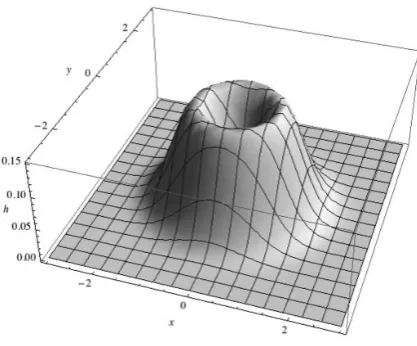
Fig. 4. Radial Weibull Distribution (m= 3, λ= 0.5)

From Eq.4, we can convert from Polar to Cartesian coor-dinates:

g(x, y) = λm

2π( √

x2_+y2₎m₋2_exp{_−λ(√_x2_+y2₎m}

(x, y, λ, m >0). (5)

Here,λ= 1/ηm_{(Figure 4).}

Assuming that each transmitter station observes indepen-dent measurements, the likelihood based on the data set is calculated as follows:

L(λ1, m1, ..., λK, mK) = K ∏ i=1 ni ∏ j=1

λimi

2π ( √

(xij−ci1)2+ (yij−ci2)2)m−2

exp [

−λi{

√

(xij−ci1)2+ (yij−ci2)2}m

] . (6)

Here, K is the number of stations and for each station i, the sample size is ni. The observed data set for station i

is (xij, yij). The coordinates(ci1, ci2)are given transmitter

station positions (Figure 1).

We calculate the estimates of x−y location parameters by maximizing the joint estimated likelihoods:

g(α, β) =

K

∏

i=1

ˆ λimˆi

2π {

(α−ci1)2+ (β−ci2)2

}miˆ 2 −1

×exp [

−_λˆ_i{_(α−ci1)2

+ (β−ci2)2

}miˆ 2 ]

(7)

The MLE of the TAG location is obtained from solving numerically the following simultaneous equations:

F = ∂logg

∂α =

K

∑

i=1

[ _{( ˆm}

i−2)(α−ci1)

(α−ci1)2+ (β−ci2)2 −_λˆ_{imˆi(α−ci1)}{_(α−ci1)2

+ (β−ci2)2

}miˆ 2 −1]

= 0

(8)

The asymptotic variance of thex-location is as follows:

AV ar [

α( ˆmi,λˆi,· · · ,mˆK,ˆλK)] =hT11Σˆh11

hT11=

( _∂α ∂mˆi

, ∂α ∂λˆi

,· · ·, ∂α ∂mˆK

, ∂α ∂λˆK

)

(9)

Here we note that the tedious calculations are needed for the differentiations by the theorem on implicit functions for maximization. Similarly, asymptotic variance of the y -location is as follows:

AV ar [

β( ˆmi,λˆi,· · ·,mˆK,λˆK)] =hT22Σˆh22

hT22=

( _∂β ∂mˆi

, ∂β ∂ˆλi

,· · ·, ∂β ∂mˆK

, ∂β ∂λˆK

)

(10)

Then, the asymptotic covariance matrix becomes

ACov[( ˆα,βˆ)] =HTΣˆH HT =

( _∂α

∂mˆi,

∂α ∂λˆi

,· · ·,_∂∂α_mˆ

K,

∂α ∂λˆK

∂β ∂mˆi,

∂β ∂λˆi

,· · ·,_∂∂β_mˆ

K,

∂β ∂λˆK

)

(11)

Here we note that the following notation should be used.

∂α ∂mˆi

= D(F, G) D(βmˆi

/∆

∂α

∂λˆi

=D(F, G) D(βˆλi

/∆

∂β ∂mˆi

= D(F, G) D(αmˆi

/∆

∂β

∂λˆi

=D(F, G) D(αˆλi

/∆

D= D(F, G)

D(α, β) (f or i= 1, ..., K) (12)

The above results come from the theorem on implicit functions. Finally we can obtain the confidence region by the following inequality equation.

(x−α, yˆ −β)[ˆ HTΣˆH]−1 (

x−αˆ y−βˆ )

≤χ2₂(p) (13)

The asymptotic covariance matrix needed for calculation of Eq.13 is as follows:

Σ =   

I₁−1 · · · 0 ..

. . .. ... 0 · · · I_K−1

  

I_i−1= 6 niπ2

×



 m

2

i miλi(γ+ logλ−1)

miλi(γ+ logλ−1) λ2i{1 + (γ−2)γ+π

2

+2 logλi(γ+ logλi−1)}

 

(14)

B. Radial Extreme Value Distribution

In the NLoS case, we can assume that the minimum value of the observed signals is the true distance between the transmitter and receiver (Figure 5). It is reasonable to assume that extreme value distribution is suitable for the NLoS data case. The extreme value distribution of the 3-parameter Weibull distribution is formulated as follows [18]:

Fz(z) = 1− {1−Fx(z)}n

= 1− [

exp {

−(z

η )m}]n

= 1−exp {

−( z

η/nm1 )m}

(15)

IAENG International Journal of Applied Mathematics, 48:2, IJAM_48_2_01

True distance from transmitter

NLoS bias

Mode value of Weibull distribution

Fig. 5. ToA data NLoS bias

where z = min(X1, X2, ..., Xn). The shape and scale

parameters of the extreme value Weibull distribution are m and ηn−m1, respectively. The shape and scale parameters are estimated from the radial Weibull distribution parameters (Eq.5). Considering the circular extreme value distribution, we can rewrite Eq.15 as follows:

Fz(r, θ) =

1 2π

[ 1−exp

{

−( r

η/nm1 )m}]

(r, η, m >0, 0≤θ <2π). (16)

From Eq.16, we can convert from Polar to Cartesian coordi-nates, same as in Eq.5, as follows:

h(x, y) =

1

2π√x2_+y2

[ 1−exp

{

−(√x2+y2

η/nm1

)m}]

(x, y, η, m >0). (17)

Using a similar procedure as in Eq.6, and assuming that each transmitter station observes independent measurements, the likelihood based on the data set is calculated as follows:

L(η1, m1, g1, ..., ηK, mK, gK) = K

∏

i=1

ni ∏

j=1

1

2π√(xij−ci1)2+ (yij−ci2)2

[ 1−exp

{

−(√(xij−ci1)2+ (yij−ci2)2−gi

ηi/n

1

mi

)mi}]

(18)

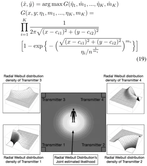
It is reasonable to assume that the highest probability location(ˆx,y)ˆ is the estimated location of the subject (Figure 6). The highest probability location from the likelihood

function is calculated as follows:

(ˆx,y) = arg maxˆ G(ˆη1,mˆ1, ...,ηˆK,mˆK)

G(x, y;η1, m1, ..., ηK, mK) = K

∏

i=1

1

2π√(x−ci1)2+ (y−ci2)2

[ 1−exp

{

−(√(x−ci1)2+ (y−ci2)2

ηi/n

1

mi

)mi}]

(19)

Fig. 6. Location estimation based on radial Weibull distribution

Calculation of maximizing the joint estimated likelihoods is same as the radial weibull distribution case.

In the next section, a comparison of simulation result of the two methods is presented.

IV. SIMULATION DETAILS AND RESULTS

To demonstrate the effectiveness of the two methods, we carried out a simulation experiments.

We considered the 10.0 m×10.0 m space chamber, four transmitters at c1 = (0,0),c2 = (10,0), c3 = (0,10), and

c4= (10,10). We generated the observation signal from the

Weibull distribution random number Xi ∼W eibull(m, λ),

where Xi are the random numbers at station i, m is the

shape parameter, λ is the scale parameter calculated from λ=l0/Γ(1+_m1),l0is the location parameter calculated from

l0=

√

(α−ci,1)2+ (α−ci,2)2, andα, β are the receiver’s

location. The number of random number generation was set toN = 100. We estimated the radial extreme value Weibull distribution parameters η,ˆ mˆ from the proposed method and estimated the receiver’s location.

For the simulation, the receiver’s locations were at(5,5), (1,1),(5,2.5), and(2.5,2.5).

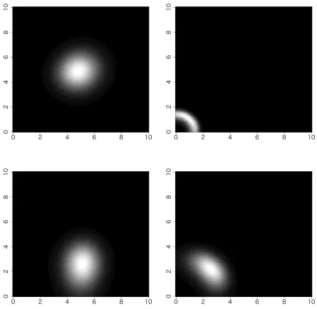
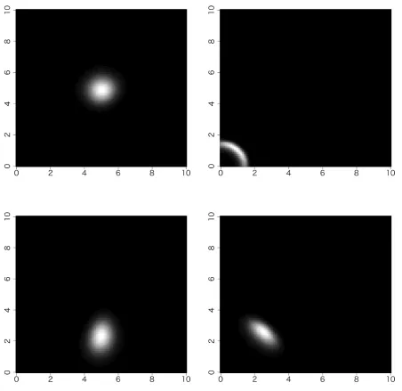
Figure 7 shows the radial Weibull distribution’s marginal likelihood in static experiment at receiver location (5,5), (1,1),(5,2.5),(2.5,2.5).

In Figure 7, the upper left figure is location(5,5), upper right figure is location (1,1), lower left figure is location (5,2.5), and lower right figure is location (2.5,2.5). The figure color indicates the marginal likelihood value, and light tone indicates high probability. The black circle in the light tone area is the receiver location.

Figure 8 shows the radial extreme value Weibull distri-bution’s marginal likelihood in static experiment at receiver

IAENG International Journal of Applied Mathematics, 48:2, IJAM_48_2_01

Fig. 7. Radial Weibull distribution’s marginal likelihood in static experiment at receiver location(5,5)(upper left),(1,1)(upper right),(5,2.5)(lower left), and(2.5,2.5)(lower right).

location (5,5), (1,1), (5,2.5), (2.5,2.5) as same as the Figure 8.

Table I shows average error distance and standard devia-tion (SD) of two methods. From Table I, radial extreme value Weibull distribution has high accuracy than radial Weibull distribution based approach.

TABLE I

AVERAGE ERROR DISTANCE AND STANDARD DEVIATION(SD)OF TWO METHODS

Average error distance [m] SD

Weibull 0.29 0.49

extreme value Weibull 0.15 0.24

From Figure 7, 8, Table I, the radial extreme value Weibull distribution based method precisely estimated the location of the subject during simulation.

V. CONCLUSIONS

In this article, we validated the performance of an in-door location estimation model based on the radial Weibull distribution, radial extreme value Weibull distribution. The simulation result suggest that radial extreme value based model can accurately estimate the subject’s spatial locations. In next phase, we will compare our methods with other state-of-the-are indoor location estimation methods, and eval-uate its performance. The computational cost of our method is lower than that of Okusa and Kamakura’s method [16]; however, its applicability for practical use is limited. Therefore, to address this limitation, we intend to review the location estimation process, especially(ˆx,y)ˆ estimation from marginal likelihood of radial extreme value obtained from the Weibull distribution. In addition, we intend to implement the indoor location estimation system based on the proposed method and demonstrate its applicability.

IAENG International Journal of Applied Mathematics, 48:2, IJAM_48_2_01

Fig. 8. Radial extreme value Weibull distribution’s marginal likelihood in static experiment at receiver location(5,5)(upper left),(1,1)(upper right),

(5,2.5)(lower left), and(2.5,2.5)(lower right).

REFERENCES

[1] Akaike, H. (1973). Information theory and an extention of the maxi-mum likelihood principle.,Int’l. Symp. Inf. Theory, pp.267–281. [2] Caffery Jr, J. J. (2000). A new approach to the geometry of TOA

location.IEEE Vehicular Technology Conference,52, 4, pp.1943–1949. [3] Chan, Y. T., Tsui, W. Y., So, H. C. & Ching, P. C. (2006). Time-of-arrival based localization under NLOS conditions. IEEE Trans. Vehicular Technology,55, 1, pp.17–24.

[4] Fujita,T., Ohtsuki, T. & Kaneko, T. (2007). Low Complexity TOA Localization Algorithm for NLOS Environments.Research paper of IPS, 15, pp.69-74.

[5] He, J., Geng, Y.,& Pahlavan, K. (2012). Modeling indoor TOA ranging error for body mounted sensors.IEEE Int’l Symp. Personal Indoor and Mobile Radio Communications (PIMRC), pp.682–686).

[6] Herrera, J. C., Hinkenjann, A., Ploger, P. G., & Maiero, J. (2013). Robust indoor localization using optimal fusion filter for sensors and map layout information. Proc. IEEE Conf. Indoor Positioning and Indoor Navigation, pp.1–8.

[7] Ikeda, T., Kawamoto, M., Sashima, A., Tsuji, J., Kawamura, H., Suzuki, K., & Kurumatani, K. (2014). An Indoor Autonomous Po-sitioning and Navigation Service to Support Activities in Large-Scale Commercial Facilities.Serviceology for Services, pp.191–201. [8] Kaemarungsi, K., & Krishnamurthy, P. (2004). Properties of indoor

received signal strength for WLAN location fingerprinting.IEEE Conf. In Mobile and Ubiquitous Systems: Networking and Services,pp.14– 23).

[9] Kamakura, T., & Okusa, K. (2013) Estimates for the spatial locations of the indoor objects by radial distributions.Proc. ISI World Statistics Congress 2013 (ISI2013),CPS109, pp.3417–3422.

[10] Knapp, C. H., & Carter, G. C. (1976). The generalized correlation method for estimation of time delay.IEEE Trans. Acoustics, Speech and Signal Processing,24,4, pp.320–327.

[11] Li, N., & Becerik-Gerber, B. (2011). Performance-based evaluation of RFID-based indoor location sensing solutions for the built environ-ment.Advanced Engineering Informatics,25, 3, pp.535–546. [12] Liu, H., Darabi, H., Banerjee, P., & Liu, J. (2007). Survey of wireless

indoor positioning techniques and systems.IEEE Trans. Systems, Man, and Cybernetics, Part C: Applications and Reviews,37, 6, pp.1067– 1080.

[13] Martin, W. (2014). Indoor Location-Based Services - Prerequisites and Foundations. Springer International Publishing, ISBN: 978-3-319-10698-4.

[14] Moses, R. L., Krishnamurthy, D., & Patterson, R. M. (2003). A self-localization method for wireless sensor networks.EURASIP Journal on Applied Signal Processing, pp.348-358.

[15] Niculescu, D. & Nath, B. (2003). Ad hoc positioning system (APS) using AOA.INFOCOM,3, pp.1734–1743.

IAENG International Journal of Applied Mathematics, 48:2, IJAM_48_2_01

[16] Kosuke Okusa, and Toshinari Kamakura, “Indoor Location Estimation based on the Statistical Spatial Modeling and Radial Distributions,” Lecture Notes in Engineering and Computer Science: Proceedings of The World Congress on Engineering and Computer Science 2015, 21-23 October, 2015, San Francisco, USA, pp.835–840.

[17] Okusa, K. & Kamakura, T. (2015). Indoor location estimation based on the RSS method using radial log-normal distribution.Proc. 16th IEEE Int. Symp, Comput. Intelligence and Informatics (CINTI2015), pp.29-34.

[18] Kosuke Okusa, and Toshinari Kamakura, “Statistical Indoor Location Estimation for the NLoS Environment Using Radial Extreme Value Weibull Distribution,” Lecture Notes in Engineering and Computer Science: Proceedings of The World Congress on Engineering 2017, 5-7 July, 2017, London, U.K., pp.555–560

[19] Patwari, N., Hero III, A. O., Perkins, M., Correal, N. S., & O’dea, R. J. (2003). Relative location estimation in wireless sensor networks. IEEE Trans. Signal Processing,51, 8, pp.2137–2148.

[20] Patwari, N., Ash, J. N., Kyperountas, S., Hero III, A. O., Moses, R. L., & Correal, N. S. (2005). Locating the nodes: cooperative localization in wireless sensor networks.Signal Processing Magazine, 22, 4, pp.54–69.

[21] Robinson, M., & Psaromiligkos, I. (2005, March). Received signal strength based location estimation of a wireless LAN client. In Wireless Communications and Networking Conference, 2005 IEEE (Vol. 4, pp. 2350-2354). IEEE.

[22] Roos, T., Myllymaki, P., Tirri, H., Misikangas, P. & Sievnen, J. (2002). A probabilistic approach to WLAN user location estimation. International Journal of Wireless Information Networks,9, 3, pp.155– 164.

[23] Shen, J., Molisch, A. F. & Salmi, J. (2012). Accurate passive location estimation using TOA measurements.IEEE Trans. Wireless Commu-nications,11, 6, pp.2182–2192.

[24] Taponecco, L., D’Amico, A. A. & Mengali, U. (2011). Joint TOA and AOA estimation for UWB localization applications.IEEE Trans. Wireless Communications,10, 7, pp.2207–2217.

[25] Venkatraman, S., Caffery Jr, J., & You, H. R. (2004). A novel TOA lo-cation algorithm using LOS range estimation for NLOS environments. IEEE Trans. Vehicular Technology,53, 5, pp.1515–1524.

[26] Watabe, T. & Kamakura, T. (2010). Localization algorithm in the indoor environment based on the ToA data, Australian Statistical Conference 2010 Program and Abstracts, p. 243.

[27] Yamada,I., Ohtsuki,T., THisanaga, T. and Zheng, L. (2008). An indoor position estimation method by maximum likelihood algorithm using received signal strength.SICE J. Control, Measurement, and System Integration,1, 3, pp.251–256.

IAENG International Journal of Applied Mathematics, 48:2, IJAM_48_2_01