TAR(p)/ARCH(1) Process with an Arbitrary
Threshold: Guaranteed Parameter Estimation and
Change-Point Detection
Sergei Vorobeychikov, Yulia Burkatovskaya and Ekaterina Sergeeva
Abstract—A sequential method of unknown autoregressive
parameters estimation of TAR(p)/ARCH(1) model with an arbitrary threshold is presented. This procedure is based on the construction of the special stopping rule and weights for weighted least square estimation method, allowing guarantee the prescribe accuracy of the estimation. Also a sequential pro-cedure of change point detection is proposed. Upper bounds for its basic characteristics, such as the probability of false alarm and the delay probability, are obtained. The ergodicity region of TAR(2)/ARCH(1) model is studied and asymptotic properties of the proposed method for ergodic TAR(p)/ARCH(1) process are investigated.
Index Terms—AR/ARCH, guaranteed parameter estimation,
change point detectionAR/ARCH, guaranteed parameter esti-mation, change point detectionT
I. INTRODUCTION
Threshold autoregressive (TAR) models proposed by Tong [1] definitely are one of the most popular classes of nonlinear time series models for conditional mean, because they do not only provide a better fit than linear models, but also reveal a strictly nonlinear behavior (e.g. limit cycles, jump resonance, harmonic distortion) which linear models cannot duplicate [2]. Though sometimes such models have to be completed by a specification of the conditional variance. ARCH/GARCH type models first introduced by Engle [3] are often considered for the conditional variance. One of the most popular applications of the models is analysis and modeling of stock market. In particular, they are used to describe the volatility. A lot of authors note that the classical ARCH/GARCH models do not explain some peculiarities of the volatility behavior, such as asymmetry and response for news. Consequently, rather complicated models based on ARCH/GARCH are proposed and used. Sidorov and others in [4] describe volatility by GARCHJumps models with two separate components (normal and unusual news), which cause two types of innovation (smooth and jump-like
Manuscript received 12 July, 2016. This paper is supported by The National Research Tomsk State University Academic D.I. Mendeleev Fund Program (NU 8.1.55.2015 L) in 2014–2015 and by RFBR Grant 16-01-00121.
S. Vorobeychikov is with the Department of Applied Mathematics and Cybernetics and International Laboratory of Statistics of Stochastic Pro-cesses and Quantitative Finance, Tomsk State University, 36 Lenin Prospekt, 634050 Tomsk, Russia, e-mail: [email protected].
Yu. Burkatovskaya is with the Institute of Cybernetics, Tomsk Polytechnic University, 30 Lenin Prospekt, 634050 Tomsk, Russia; Department of Ap-plied Mathematics and Cybernetics and International Laboratory of Statistics of Stochastic Processes and Quantitative Finance, Tomsk State University, 36 Lenin Prospekt, 634050 Tomsk, Russia, e-mail: [email protected].
E. Sergeeva is with the Institute of Cybernetics, Tomsk Polytech-nic University, 30 Lenin Prospekt, 634050 Tomsk, Russia; e-mail: sergeeva e [email protected].
innovations). The first component is the GARCH process, and the second one reflects the result of unexpected events and describe jumps in volatility. Guo and Cao in [5] propose a new smooth transition GARCH model, which allows for an asymmetric response of volatility to the size and sign of shocks, and an asymmetric transition dynamics for positive and negative shocks. The authors apply the model to the em-pirical financial data: the NASDAQ index and the individual stock IBM daily returns. TAR/ARCH models also allows us to describe some non-linear effects, such as clustering and different behavior subject to the sign of a stock return.
Estimators of the unknown parameters based on the idea of the usage of a special stopping rule in order to guarantee precisely their quality in a special sense were first proposed by Wald in [6] and are also very popular. So, Lee and Sriram in [7] proposed a sequential procedure for estimation of TAR(1) parameters, which allows one to construct least squares asymptotically risk efficient estimator. Sriram in [8] used sequential sampling methods to construct confidence intervals for unknown parameters with the fixed size and prescribed coverage probability. Konev and Galtchouk in [9] proposed the sequential least square estimator with the stopping rule determined by the trace of the observed Fisher information matrix, which is asymptotically normally dis-tributed in the stability region. In [10] we developed a se-quential procedure for the estimation of unknown parameters of the TAR(1)/ARCH(1) process, which can guarantee the precise accuracy of estimators.
The problem of the change point detection for autore-gressive processes with conditional heteroskedasticity is well known and extremely interesting. With different assumption and for different types of models such problem was recently considered for example by Vorobeychikov and others in [10], Fryzlewicz and Subba Rao in [11], Na, Lee and Lee in [12]. Properties of commonly used algorithms are studied asymptotically or by simulations, as theoretical investigation is extremely complicated or hardly ever possible. The usage of the special stopping rule for the least squares estimators with the guaranteed accuracy of unknown parameters allows us to investigate both asymptotic and non-asymptotic proper-ties of algorithms, such as false alarm and delay probabiliproper-ties. This paper proposes the guaranteed weighted least square estimators of unknown autoregressive parameters of the TAR(p)/ARCH(1) process with an arbitrary threshold. Asymptotic properties for the estimators are considered and the upper bounds for the standard deviation (asymptotic and non-asymptotic) are constructed. The authors present the procedure of change point detection with guaranteed characteristics for this process.
IAENG International Journal of Applied Mathematics, 46:3, IJAM_46_3_11
II. PROBLEMSTATEMENT
We consider the TAR(p)/ARCH(1) autoregressive process specified by the equation
xk =XkΛ11{xk−1≥a}+X
T
kΛ21{xk−1<a}
+qω+α2x2 k−1ξk; Xk = [xk−1, ..., xk−p];
Λj= [λj
1, ..., λjp]T, j= 1,2,
(1)
where{ξk}k≥0 is a sequence of independent identically dis-tributed random variables with zero mean and unit variance, ω > 0, 0 < α2 <1, ais an arbitrary known constant. So, the process under consideration is thep-order autoregressive process with ARCH noise and the autoregressive parame-ters depending on the previous value of the process. The value of the parameter vector Λ = [Λ1,Λ2] changes from µ = [µ1
1, ..., µ1p, µ21, ..., µ2p] to β = [β11, ..., βp1, β12, ..., βp2] at the change pointθ. The parameters values before and afterθ are supposed to be unknown. The difference betweenµand β satisfies the condition
(µj−βj)T(µj−βj)≥∆, j= 1,2, (2) where∆is the known value defining the minimum difference between the parameters before and after the change point. The problem is to detect the change point θ from the observations xk.
In [19] and [20], we proposed to detect the instant of the parameters change in the autoregressive process by making use of guaranteed sequential estimators. The sequence of estimators is constructed and the estimators obtained on different time intervals were compared. In paper [21], we applied this approach to more complicated TAR(p)/ARCH(1) model with the unbounded noise variance. In this paper, we extend our approach to TAR(p)/ARCH(1) model with an arbitrary threshold. The ergodicity region of the process is investigated. Besides, more precise asymptotic results are obtained.
III. ERGODICITY OF THEPROCESS
For investigation of asymptotic properties of estimators of unknown parameters of the given models it is important to obtain necessary and sufficient conditions for ergodicity or even strongly for geometric ergodicity of such models . There are distinguished three main approaches to establish geo-metrical ergodicity in nonlinear conditionally heterockedas-tic autoregression [2]. The first approach is based on the assumption that the linear regression part becomes main part for the stability research due to the usage of infinite number of values of the process considered; the assumption that the radius of the companion matrix of this linear regression part is less than one [13], [14] for the AR/ARCH model. The second one uses the concept of the Lyapunov exponent for the AR/ARCH [15] and the TAR/ARCH [16] and allows to obtain geometric ergodicity within more general assumptions in much larger parameter space than in [13], [14] but the assumptions appear much more difficult to validate. The last one is the approach, which was proposed first by Liebscher [17] and then extended for AR/ARCH model [3], based on the concept of the joint spectral radius of a set of matrices and also allows to obtain the geometric ergodicity in lager regions of parameter space than [13], [14].
In this paper, we obtained sufficient conditions for ergod-icity of process (1) based on one of the theorems given by Mein and Tweedie [22]. We can reduce proving geometric ergodicity of a Markov chain{Xn}by verifying the follow-ing condition: there is a positive test functiong(X)such as and a compactK such as
a)E[g(Xk+1)|Xk =X]< g(X)−c, c >0, X /∈K;
b)E[g(Xk+1)|Xk =X]< R <∞, X∈K;
(3)
The main problem of this approach is the choice of the functiong(X). Let us choose it as a linear function of the X. For the TAR(2)/ARCH(1) process we can write it in the form
g(Xk+1) =C1+x + k +C
−
1x
−
k +C + 2x
+ k−1+C
−
2x
−
k−1, whereC1+,C1−,C2+,C2− are some positive constants,
x+= max{x,0}, x−= max{−x,0}.
We choose the compactK= [−M, M]×[−M, M], where M >|a|.
At first, we consider condition (3a). Forxk−1> M using (1) we obtain
g(Xk+1) =C1+
λ11xk−1+λ12xk−2+ q
ω+α2x2 k−1ξk
+
+C1−λ1
1xk−1+λ12xk−2+ q
ω+α2x2 k−1ξk
−
+C2+xk−1;
Consequently (here and then,X= (xk−1, xk−2)), E[g(Xk+1)|Xk=X]
=C1+ λ11xk−1+λ12xk−2
+∞
Z
Dk
f(x)dx
+C1+
q
ω+α2x2 k−1
+∞
Z
Dk
xf(x)dx
−C1− λ11xk−1+λ12xk−2
Dk
Z
−∞
f(x)dx
−C11qω+α2x2 k−1
Dk
Z
−∞
xf(x)dx+C2+xk−1;
Dk=
−λ1
1xk−1−λ12xk−2 q
ω+α2x2 k−1
.
Heref(x)is the density of distribution of the noiseξk. By introducing the following notations
+∞
Z
Dk
xf(x)dx=Fk1, +∞
Z
Dk
xf(x)dx=Fk2,
and taking into account that Eξk = 0, we can rewrite the
IAENG International Journal of Applied Mathematics, 46:3, IJAM_46_3_11
last equation in the form
E[g(Xk+1)|Xk =X] =C1+ λ 1
1xk−1+λ12xk−2
Fk1
+C1+qω+α2x2 k−1F
2 k
−C1− λ11xk−1+λ12xk−2
(1−Fk1) −C1−qω+α2x2
k−1(−F 2 k) +C
+ 2xk−1
= (C1++C1−) λ1
1xk−1+λ21xk−2Fk1
−C1− λ1
1xk−1+λ12xk−2
+C2+xk−1
+(C1++C1−)qω+α2x2 k−1F
2 k.
Note that if the functionf(x)is symmetric than
0≤Fk2≤
∞
Z
0
xf(x)dx=D. (4)
The function g(X)has the following form g(X) =
C1+xk−1+C2+xk−2, if xk−2>0; C1+xk−1−C2−xk−2, if xk−2≤0. Hence, forxk−2>0
E[g(Xk+1)|Xk=X]−g(X)
= (C1++C1−)λ1
1xk−1Fk1−C
−
1λ11xk−1+C2+xk−1
−C1+xk−1 + (C1++C
−
1) q
ω+α2x2 k−1F
2 k
+(C1++C1−)λ12xk−2Fk1−C
−
1λ 2
1xk−2−C2+xk−2. Asxk−1andxk−2can take any value, to fulfill condition (3a) the last expression should satisfy the following inequalities
1) (C1++C1−)λ11xk−1Fk1−C1−λ 1
1xk−1+C2+xk−1
−C1+xk−1+ (C1++C
−
1) q
ω+α2x2
k−1Fk2<0;
2) (C1++C1−)λ1
2xk−2Fk1−C
−
1λ 2
1xk−2−C2+xk−2≤0. The further reasonings depend on the signs of the parameters λ1
1,λ12. Consider all possible cases.
• λ1
1>0. In expression 1), the first summand is positive, andF1
k <1; besides, the last summand is also positive and F2
k < D, whereDis defined in (4). So, to fulfill 1) we need
(C1++C1−)λ11xk−1−C1−λ 1
1xk−1+C2+xk−1
−C1+xk−1+ (C1++C1−) q
ω+α2x2
k−1D <0; hence, we obtain the following condition of ergodicity
α < C + 1(1−λ
1 1)−C
+ 2
(C1++C1−)D .
• λ1
1 ≤ 0. In expression 1), the first summand is non-positive; so, to fulfill 1) we need
−C1−λ11xk−1+C2+xk−1−C1+xk−1
+(C1++C1−)qω+α2x2
k−1D <0; hence, we obtain the following condition of ergodicity
α < C
−
1λ11+C + 1 −C
+ 2
(C1++C1−)D . To fulfill it, we need the following condition
C1−λ11+C1+−C2+>0. Introducing the following notations
C1− C1+ =t,
C2+ C1+ =s,
we can rewrite the ergodicity conditions forλ1
1 in the form α < (1−λ
1 1)−s
(1 +t)D , λ 1 1>0;
α < tλ 1
1+ 1−s
(1 +t)D . λ 1 1<0;
(5)
Consider now condition 2). Taking into account that xk−2>0, we obtain
(C1++C1−)λ12Fk1−C1−λ12−C2+≤0.
• λ1
2 > 0. The first summand is positive; hence, the condition takes the form
(C1++C1−)λ12−C1−λ12−C2+≤0, consequently,
λ12≤ C
+ 2 C1+ =s.
• λ1
2 ≤0. The first summand is non-positive; hence, the condition takes the form
−C1−λ12−C2+≤0, consequently,
λ12≥ −C
+ 2 C1− =−
s t.
Consider now the casexk−2<0. Following the same line of reasoning, we obtain the ergodicity conditions
1) (C1++C1−)λ11xk−1Fk1−C
−
1λ 1
1xk−1+C2+xk−1
−C1+xk−1+ (C1++C
−
1 ) q
ω+α2x2 k−1F
2 k <0;
2) (C1++C1−)λ12xk−2Fk1−C
−
1λ 1
2xk−2+C2−xk−2≤0. Condition 1) is the same, and condition 2) can be rewritten in the form
−(C1++C1−)λ12Fk1+C1−λ12−C2−≤0 • λ1
2 >0. The first summand is non-positive; hence, the condition takes the form
C1−λ12−C2− ≥0, consequently,
λ12≤C
−
2 C1−.
• λ12 ≤ 0. The first summand is positive; hence, the condition takes the form
−(C1++C1−)λ12+C1−λ12−C2−≤0
consequently,
λ12≥ −C
−
2 C1+. Introducing the following notation
C2− C1+ =q,
we can rewrite the ergodicity conditions forλ1
2 in the form
maxn−s
t,−q
o
≤λ12≤minns,q t
o
. (6)
IAENG International Journal of Applied Mathematics, 46:3, IJAM_46_3_11
Forxk−1<−M using (1) we obtain g(Xk+1) =C1+
λ2
1xk−1+λ22xk−2+ q
ω+α2x2 k−1ξk
−C2−xk−1; Consequently,
E[g(Xk+1)|Xk =X]
= (C1++C1−) λ21xk−1+λ22xk−2
Fk1
−C1− λ2
1xk−1+λ22xk−2−C2−xk−1
+(C1++C1−)qω+α2x2 k−1F
2 k.
The function g(X)has the following form g(X) =
−C1−xk−1+C2+xk−2, ifxk−2>0;
−C1−xk−1−C2−xk−2, ifxk−2≤0. Hence, for xk−2 >0 the last expression should satisfy the following conditions
1) (C1++C1−)λ21xk−1Fk1−C
−
1λ 2
1xk−1−C2−xk−1
+C1+xk−1+ (C1++C
−
1) q
ω+α2x2 k−1F
2 k <0;
2) (C1++C1−)λ22xk−2Fk1−C
−
1λ 2
2xk−2−C2+xk−2≤0. Forxk−2<0 the conditions are
1) (C1++C1−)λ21xk−1Fk1−C
−
1λ 2
1xk−1−C2−xk−1
+C1−xk−1+ (C1++C
−
1) q
ω+α2x2 k−1F
2 k <0;
2) (C1++C1−)λ22xk−2Fk1−C
−
1λ 2
2xk−2+C2−xk−2≤0. Conditions 2) are practically the same as in the previous case xk−1 > M, we only need to use λ22 instead of λ12; so, we obtain
maxn−s
t,−q
o
≤λ22≤minns,q t
o
. (7)
Consider now condition 1) for different signs ofλ2 1.
•λ2
1≥0. The first summand in 1) is non-positive; so, the condition has the form
−C1−λ21xk−1−C2−xk−1+C1−xk−1
+(C1++C1−)qω+α2x2 k−1F
2 k <0
and implies the inequality α < −C
−
1 λ21+C1−−C2−
(C1++C1−)D .
• λ2
1 < 0. The first summand in 1) is positive; so, the condition has the form
(C1++C1−)λ21xk−1−C1−λ 2
1xk−1−C2−xk−1+C1−xk−1
+(C1++C1−)qω+α2x2 k−1F
2 k <0
and implies the inequality
α < C + 1λ
2
1+C1−−C
−
2
(C1++C1−)D .
So, we obtain the ergodicity conditions forλ11 in the form α < t(1−λ
2 1)−q
(1 +t)D , λ 2 1≥0;
α < λ 2 1+t−q
(1 +t)D , λ 2 1<0.
(8)
Finally, by making use (5) and (6) we combine all ergod-icity conditions for the parameterα
α < (1−λ 1 1)−s
(1 +t)D , λ 1 1>0;
α < tλ 1
1+ 1−s
(1 +t)D , λ 1 1≤0;
α < t(1−λ 2 1)−q
(1 +t)D , λ 2 1≥0;
α < λ 2 1+t−q
(1 +t)D , λ 2 1<0.
(9)
Note that the upper bound for αshould be positive. Taking into account thatt >0 we obtain additional conditions
(1−λ11)−s >0, λ1 1>0; tλ11+ 1−s >0, λ1
1≤0; t(1−λ21)−q >0, λ21≥0;
λ21+t−q >0, λ2 1<0;
(10)
By making use (8) and (7) we combine all ergodicity conditions for the parameterλl
2
maxn−s
t,−q
o
≤λl2≤minns,q t
o
. (11)
To obtain the widest ergodicity region for α, we should minimizesandqtaking into account conditions (11). There can be several cases subject to the parametersλl
2.
Case 1:0≤λ2
2< λ12. In this case, condition (11) has the form
λ12≤minns,q t
o
,
and minimum values of the constants ares=λ1
2,q=tλ12. Note that the case 0 ≤ λ1
2 < λ22 is in fact the same; we only need to replace further λ1
2 by λ22. Using this, we can construct the ergodicity region forαsubject to the signs of the parametersλl
1. λ1
1>0,λ21≥0. The ergodicity region takes the form α <min
1
−λ1 1−λ12
(1 +t)D ,
t(1−λ2 1−λ12)
(1 +t)D
(12) with the additional conditions
1−λ1
1−λ12>0;
1−λ2
1−λ12>0, which can be generalized in the form
λj1+λl2<1, j, l∈ {1,2}. (13) We obtain the widest region if the parameter t satisfies the equation
1−λ11−λ12=t(1−λ21−λ12).
In this case both upper bound constants for α are equal; hence, choosing minimum between them, we obtain the maximum value of the upper bound. By expressing t from this and using it in (12), we obtain
α < (1−λ 1
1−λ12)(1−λ21−λ12)
(2−λ1
1−λ21−2λ12)D
. (14)
Due to condition (13), the right hand side of (14) is positive. λ1
1>0,λ21<0. The ergodicity region takes the form α <min
1−λ1 1−λ12
(1 +t)D , λ2
1+t−tλ12
(1 +t)D
(15)
IAENG International Journal of Applied Mathematics, 46:3, IJAM_46_3_11
with the additional conditions
1−λ1
1−λ12>0
which has already obtained in (13). The parametert provid-ing the biggest region of ergodicity satisfies the equation
1−λ11−λ12=λ21+t−tλ12.
By expressing tfrom this and using it in (15), we obtain α < (1−λ
1
1−λ12)(1−λ12)
(2−λ1 1−λ
2 1−2λ
1 2)D
. (16)
Due to condition (13), the right hand side of (16) is positive. Similarly, we can consider two remaining cases.
λ11≤0,λ21≥0. The ergodicity region is α < (1−λ
2
1−λ12)(1−λ12)
(2−λ1
1−λ21−2λ12)D
(17) if conditions (13) fulfill.
λ11≤0,λ21<0. The ergodicity region is α < (1−λ
1
2)2−λ11λ21
(2−λ1
1−λ21−2λ12)D
(18) with the additional conditions
(1−λl2)2−λ11λ21>0. (19) So, forλ1
2≥0andλ22≥0combining (13)–(19) we obtain the following ergodicity region
λl2≥0, l∈ {1,2};
λj1+λl
2<1, j, l∈ {1,2}; λ1
1λ21<(1−λl2)2, l∈ {1,2}; α < min{A1, A2, A3, A4}
(2−λ1
1−λ21−2 max{λ12, λ22})D
=α∗,
(20)
where
A1= (1−λ11−max{λ12, λ22})(1−λ21−max{λ12, λ22}); A2= (1−λ11−max{λ12, λ22})(1−max{λ12, λ22}); A3= (1−λ21−max{λ12, λ22})(1−max{λ12, λ22});
A4= (1−max{λ12, λ22})2−λ11λ21.
Case 2: λ1
2< λ22≤0. In this case, condition (11) has the form
minn−q,−s
t
o
≤λ12
and minimum values of the constants are s = −tλ12, q =
−λ12. Note that the caseλ22< λ12≤0is in fact the same; we only need to replace further λ12 by λ22. Using this, we can construct the ergodicity region forαas described above for the case 1. The region has the following form
λl
2≤0, l∈ {1,2};
(1−λ1
1)(1−λ21)− λl2 2
>0, l∈ {1,2};
λj1+λl2(λ 3−j 1 +λ
l
2)<1, j, l∈ {1,2}; λ11λ21+λl2(λ11+λ21+λl2)<1, l∈ {1,2};
α < min{B1, B2, B3, B4}
(2−λ1
1−λ21−2 min{λ12, λ22})D
=α∗,
(21)
where
B1= (1−λ11)(1−λ12)− min{λ12, λ22} 2
;
B2= 1−λ11−min{λ12, λ22}(λ21+ min{λ12, λ22}); B3= 1−λ21−min{λ12, λ22}(λ11+ min{λ12, λ22}); B4= 1−λ11λ12−min{λ12, λ22}(λ11+λ21+ min{λ12, λ22}).
If we choose
M > ω
(α∗)2−α2, and
g(Xk+1) =x+k +tx−k +sx+k−1+qx−k−1,
wheres,q and t are constructed as above, subject to signs ofλj1,λl
2,j, l∈ {1,2}, condition (3a) will be fulfilled.
Case 3:λ1
2<0< λ22. In this case, evaluations andqis more difficult then in the previous one, because we should take into account not only signs of λj2 but their absolute values. As a result, we have three possible sets of values for s and q, and we should consider these sets subject to signs ofλl1, i.e., for four cases. These calculations are rather cumbersome; so, we do not consider this case in the paper. To prove condition (3b) we have to bound from above E[g(Xk+1)|Xk=X]when X∈K; we have
E[g(Xk+1)|Xk=X]
= (C1++C1−)λj1xk−1+λ j 2xk−2
Fk1
−C1−λj1xk−1+λ j 2xk−2
+C2+xk−1
+(C1++C1−)qω+α2x2 k−1F
2 k
≤(C1++C1−)|λj1|+|λj2|M
+C2+M+ (C1++C1−)√ω+α2M2D <∞. Note that when λ1
2 = λ22 = 0, the ergodicity re-gions (20) and (21) matches the one obtained in [10] for TAR(1)/ARCH(1). It differs from regions described in [18] and [14], because it includes negative values of the parame-tersλ1
1 <−1 or λ21<−1; in [18] and [14] absolute values of all parameters are less then one. Cline and Pu in [16] obtained the exact ergodicity region for more general model TAR(p)/ARCH(p), but it should be calculated numerically forp >1; in our paper, we proposed explicit expressions.
Fig. 1 demonstrates an example of an ergodic TAR(2)/ARCH(1) process behavior, and Fig. 2 presents an example of non-ergodic one. Both trajectories have cluster effect and outliers, but the latter one is more chaotic and maximum values of the process are greater then for the former one.
IV. GUARANTEED PARAMETER ESTIMATOR
Since the parameters both before and after the change point are unknown, it is logical to apply the estimators of the unknown parameters in the change point detection procedure. In this section we construct guaranteed sequential parameter estimators for the parameter vectorsΛj, j= 1,2. Such esti-mators were proposed in [20] for an autoregressive process. The main advantage of the estimators is their preassigned mean square accuracy depending on the parameter of the estimation procedure.
It should be noted that if parametersωandαare unknown then the process (1) has unknown and unbounded from above noise variance. To obtain a process with bounded noise variance we denote max{1,|xk−1|} as mk and rewrite the
IAENG International Journal of Applied Mathematics, 46:3, IJAM_46_3_11
Fig. 1. Ergodic TAR(2)/ARCH(1) process
Fig. 2. Non-ergodic TAR(2)/ARCH(1) process
process in the form
yk =Yk1Λ1+Yk2Λ2+γkξk; Yk1= 1
mk
Xk1{xk−1≥a}. Y
2 k =
1
mk
Xk1{xk−1<a};
yk= xk mk
, γk= q
w+α2x2 k−1 mk
.
(22) The noise variance of the process {yk} is bounded from above by the unknown value (ω +α2). To eliminate the influence of the unknown constant in [10] we proposed to use the special factorΓN constructed by firstN observations in the following form
ΓN =CN N X
k=1
x
k
min{1,|xk|} 2
;
CN =E N
P k=1
ξ2 k
−1
,
(23)
whereN observations are taken at the interval where all the values |xk|are sufficiently large. It was proved in [20] that
for the process AR(p) the compensating factor satisfies the following condition
E 1
ΓN
≤ 1
ω+α2. (24)
This proof can be generalized for our case with minimum changes so we omit it.
If the random variables {ξk} have standard normal dis-tribution, then the sum
N P k=1
ξk2 has χ2 distribution with N degrees of freedom. In this case
CN =
1 2N/2Γ(N/2)
+∞
Z
0
xN/2−3e−x/2dx= 1
(N−2)(N−4).
This constant is defined forN≥5.
Let us consider now a weighted least squares estimator for process (22). The process can be rewritten in the form
yk=YkΛ +γkξk; Yk = [Yk1, Yk2].
(25) So the weighted least squares estimator has the following form
ˆ
Λ =C−1(m)
m P k=N+1
vk(Yk)Tyk;
C(m) =
m P k=N+1
vk(Yk)TYk,
(26)
where0< vk≤1. According to definition (22)(Y j k)
TYi k = Opfori6=j(hereOpstands for a zero matrix of the orderp). Hence, taking into account (25), one obtains that the matrix C(m)has a block structure
C(m) =
C(1, m) Op Op C(2, m)
C−1(m) =
C−1(1, m) Op Op C−1(2, m)
C(j, M) =
m P k=N+1
vk(Ykj)TYkj, j= 1,2.
Using this result and (22), (25) one can obtain
ˆ
Λ1= [C−1(1, m)O p]
m P k=N+1
vk(Yk)Tyk
= [C−1(1, m)Op] m P k=N+1
vk(Yk)T(YkΛ +γkξk)
= [C−1(1, m)O p]
C(1, m)Λ1 C(2, m)Λ2
+[C−1(1, m)O p]
m P k=N+1
vk(Yk)Tγkξk.
Hence,
ˆ Λ1= Λ
1+C−1(1, m)η(1, m); η(1, m) =
m P k=N+1
vk(Yk1)Tγkξk. (27)
The same result can be obtained for Λˆ2. It allows us to construct estimators forΛ1 andΛ2 separately, i.e.
ˆ
Λj =C−1(j;m) Pm k=N+1
vk(Ykj)Tyk, j= 1,2. (28) The obtained estimator can be modified in order to bound the standard deviation of the estimator from above. To do so, we change the sample size m for a special random
IAENG International Journal of Applied Mathematics, 46:3, IJAM_46_3_11
stopping timeτj. Also, we use special weightsv
j,kfor every estimator.
Let H > 0 be a parameter of the estimation procedure. Further we prove that it defines the accuracy of the proposed parameter estimators. Then the estimators are constructed by using the sequential weighted least squares method and consequently can be written in the following form:
ˆ
Λj = ˆΛj(H) =C−1(j;τj) τ j
P k=N+1
vj,k(Ykj)Tyk;
C(j, M) =
m P k=N+1
vj,k(Y j k)
TYj
k, j = 1,2.
(29)
Let νmin(j, M) be the minimum eigenvalue of the matrix C(j, M). Then the stopping instantsτj =τj(H)are defined by the following conditions
τj = inf (M > N : νmin(j, M)≥H). (30) Now we consider the choice of the weights vj,k. Let the matrix C(j, M) be degenerate for M =N+ 1, ..., N+σj and C(j, σj + 1) be non-degenerated. The weights on the interval [N+ 1, N+σj] are taken in the following form:
vj,k=
1
q
ΓNYkj(Y j k)T
,
if YNj, . . . , Ykj are linearly independent;
0, otherwise.
(31)
The weights on the intervals[N+σj+ 1, τj−1]are found from the following condition:
νmin(j, k)
ΓN
=
k X
l=N+σ
v2(j, l)Ylj(Ylj)T. (32)
At the instantsτj, the weights are determined by the condi-tion:
νmin(j, τj)
ΓN
≥
τj
X
l=N+σ+1
v2(j, l)Ylj(Ylj)T;
νmin(j, τj) =H.
(33)
Theorem 1. Let the parameter vectorΛjin (1) be constant. Then the stopping timeτj (30) is finite with probability one and the mean square accuracy of estimator (29) is bounded from above
E||Λˆj(H)−Λj||2≤H+p−1
H2 . (34)
Proof. According to the definition of the instantτj (30) it is finite with probability one if
k X
l=N+σ
v2(j, l)Ylj(Ylj)T → ∞ ask→ ∞. (35)
The series converges if and only if∀ε >0 asM → ∞(see [23])
P
X
l≥M
v2(j, l)Ylj(Ylj)T ≥ε
→0. (36)
The factor Ylj(Ylj)T does not tend to zero because the absolute value of the first component is equal to
|xl−1|1[xl−1≥a]/max{1,|xl−1|} for j = 1, and it is equal
to|xl−1|1[xl−1<a]/max{1,|xl−1|}for j= 2. According to
equation (1),|xl−1|exceeds unity with a non-zero probability
and can be both greater and smaller then a; hence, the absolute value of the first component is equal to 1 with non-zero probability. So condition (36) can hold true only because of the choice of the weightsv(j, l).
Suppose that the matrix C(j, M −1) is not diagonal. According to the definition of the minimum eigenvalue of a matrix
νmin(j, M) = min x:||x||=1
(x, C(j, M)x),
where (x, y) is the scalar product of the vectors x and y. Then by using (29), we obtain
νmin(N+ 1, N)
= min
x:||x||=1(x,((C(j, M −1) +vj,M(Y j M)
TYj M)x)
= min
x:||x||=1
((x, C(j, M −1)x) +vj,M(Y j Mx)
2).
Let zM be the argument of the minimum in the above equation. According to (32), we obtain
(zM, C(j, M−1)zM) +vj,M(YMjzM)2
=νmin(j, M−1) +v2j,MY j M(Y
j M)
T.
So we have derived the quadratic equation for vj,M with roots in the form
v1,2=
1
2YMj(YMj)T h
(YMjzM)2±
√
Di;
D= (YMjzM)4
+4YMj(YMj)T[(zM, C(j, M−1)zM)−νmin(j, M−1)]. It is obvious that
(zM, C(j, M −1)zM)−νmin(j, M−1)≥0.
Thus the following two cases are possible.
Case 1. The equation has two zero roots: v1 = v2 = 0. This is possible if and only ifzM is the eigenvector of the matrix C(j, M −1) corresponding to νmin(j, M −1) and YMjzM = 0. However, the first component ofYMj depends on the random variable ξM, which is independent on the
{Ykj}k<M. Hence the vectorYMj is orthogonal to the given eigenvector of the matrixC(j, M−1)with zero probability.
Case 2. The equation has one non-positive and one positive
root. Taking the major root asvj,M, one obtains
vj,M2 Y j M(Y
j M)
T ≥ (Y j MzM)4 YMj(YMj)T
+(zM, C(j, M −1)zM)−νmin(j, M−1).
(37)
The first term in (37) is equal to YMj(YMj)Tcos4(αM)/2, where αM is the angle between Y
j
M and zM. Since YMj(YMj)T does not converge to zero, the first term converges to zero if and only ifcos(αM)→0 whenM → ∞. On the other hand, if the second term in (37) converges to zero then zM converges to the eigenvector of the matrixC(j, M−1) corresponding to νmin(j, M −1). If vj,M → 0, then the matrix C(j, M) changes slightly with the increasing M. Hence, the eigenvectors of the matrix change slightly too, and zM converges to a certain vectorz∗. Therefore, the right side of (37) converges to zero if the cosine of the angle between YMj andz∗converges to zero. However, the first component of YMj depends on xM−1 which can take any value, this cosine can be sufficiently large with non-zero probability.
IAENG International Journal of Applied Mathematics, 46:3, IJAM_46_3_11
Note that condition (36) can hold true if all eigenvalues of the matrix C(j, M −1) for certain M are equal. It is possible if and only if the matrix C(j, M −1) is diagonal. The matrixC(j, N+k) =vj,N+k(YNj+k)TYNj+k, wherekis the least number such asYN+kj is non-zero, is not diagonal. It can easily be proved that if the matrixC(j, M−1)is not diagonal, then the next matrixC(j, M)is diagonal with zero probability.
Hence, condition (36) does not hold true for TAR(p)/ARCH(1) process (1), and this implies (35).
According to (27), one can obtain
ˆ
Λj= Λj+C−1(j, τj)η(j, τj); η(j, τj) = τ
j
P k=N+1
vj,k(Ykj)Tγkξk.
By using the norm properties and (32), one obtains
||Λˆj(H)−Λj||2≤(ν
min(j, τj))−2||η(j, τj)||2
≤||η(j, τ
j)||2
H2 .
(38)
LetFk =σ{ξ1, ..., ξk} be a sigma-algebra generated by the random variables {ξ1, ..., ξk} andτj(M) = min{τj, M} is a truncated stopping instant. According to (30) the instant τj(M) satisfy the condition{τj(M) = k} ∈ Fk−1. Using
the properties of conditional expectations one obtains E||η(j, τj(M))||2
=E M P k=N+1
E[vj,k2 Ykj(Ykj)Tγk2ξk21τj≤k|Fk−1]
+2E M P k=N+2
k−1 P l=N+1
E[vj,kvj,lYkj(Y j l)
Tγ
kγlξkξl1τj≤k|Fk−1]
=E M P k=N+1
v2 j,kY
j k(Y
j
k)Tγk21τj≤kE[ξk2|Fk−1]
+2E M P k=N+2
k−1 P l=N+1
vj,kvj,lYkj(Ylj)Tγkγlξl1τj≤kE[ξk|Fk−1]. Since ξk does not depend onFk−1, the second summand is
equal to zero and one obtains
E||η(j, τj(M))||2=E τj(M)
X
k=N+1
vj,k2 Ykj(Ykj)Tγk2.
Due to the choice of the weights vj,k (31–32) one obtains
E τj
P k=N+1
v2 j,kY
j k(Y
j k)
T =E N+σ j
P k=N+1
v2 j,kY
j k(Y
j k)
T
+E τj
P k=N+σj+1
v2 j,kY
j k(Y
j k)
T ≤p−1
ΓN
+ H ΓN
.
According to (22) one can see thatγk2≤ω+α2. Note that τj(M)→τj as M → ∞, so
E||η(j, τj)||2≤(ω+α2)(H+p−1)E 1
ΓN .
Due to property (24) of the factor ΓN and inequality (38) one obtains
||Λˆj(H)−Λj||2≤H+p−1 H2 . The theorem has been proved.
Further we establish asymptotic properties of the con-structed procedures. We need the following auxiliary result.
Lemma 1. Let ξ1, . . . , ξn be independent identically
distributed standard Gaussian variables. Then for any λ1, . . . , λn, λi ≥0, λ1+. . .+λn = 1 and for sufficiently
largeC
P
λ1ξ12+. . .+λnξ2n> C ≤ P
ξ21> C . (39)
Proof. First we give the proof for the case ofn= 2. We need to minimize the function
J(λ1) =P
λ1ξ21+ (1−λ1)ξ22< C → min 0≤λ1≤1/2
. (40) Here we take into account that the variables ξ1 and ξ2 are independent identically distributed, thusJ(λ1) =J(1−λ1). We rewrite the last expression in the form
J(λ1) = C/λ1
Z
0
P
λ1y+ (1−λ1)ξ22< C f(y)dy
=
C/λ1
Z
0
P
ξ22<
C−λ1y
1−λ1
f(y)dy
=
C/λ1
Z
0 F
C−λ 1y
1−λ1
f(y)dy,
wheref(·)is the density of distribution,F(·)is the distribu-tion funcdistribu-tion of the variable ξ2i. Differentiating J(λ1), one obtains
J0(λ1) = C/λ1
Z
0 f
C−λ1y
1−λ1
C−y
(1−λ1)2 f(y)dy
=
C Z
0 f
C−λ 1y
1−λ1
C−y
(1−λ1)2 f(y)dy
−
C/λ1
Z
C f
C−λ 1y
1−λ1
y−C
(1−λ1)2
f(y)dy.
Both integrals in the last expression are positive. The second one tends to zero whenC→ ∞. Thus
lim
C→∞J 0(λ
1)≥0 ∀λ1∈[0,1/2].
Forλ1= 0 one can obtain
J0(0) =
∞
Z
0
f(C) (C−y)f(y)dy=f(C)(C−1)
IfC >1 thenJ0(0)>0, andJ(λ1)increases withλ1. For λ1= 1/2 we can obtain
J0(1/2) = 4
2C Z
0
f(2C−y)(C−y)f(y)dy
= 2
2C Z
0
f(2C−y)(2C−y)f(y)dy
−2
2C Z
0
f(2C−y)yf(y)dy= 0.
IAENG International Journal of Applied Mathematics, 46:3, IJAM_46_3_11
Here we use the change of the variable y = 2C−z in the second integral. For an arbitraryλ1∈(0,1/2]one obtains
J0(λ1) = C Z
0 f
C−λ 1y
1−λ1
C−y
(1−λ1)2 f(y)dy
− C/λ1 Z C f
C−λ1y
1−λ1
y−C
(1−λ1)2
f(y)dy.
Both integrals in the last expression are positive. The second one tends to zero whenC→ ∞. Thus
lim
C→∞J 0(λ
1)≥0 ∀λ1∈[0,1/2]. Hence using (40) one obtains
P
λ1ξ21+ (1−λ1)ξ22< C ≥ P
ξ21< C . (41) Letλ1≤. . .≤λn,λ1+. . .+λn= 1, henceλ1∈[0,1/n]. We need to prove that for sufficiently largeC
P
λ1ξ12+. . .+λnξn2> C ≥ P
ξ12< C . (42) Inequality (41) gives us this result for n= 2. Suppose that (42) holds for 2, 3, ..., n−1 summands. Then
P
λ1ξ12+. . .+λnξn2> C
= C/λ1 Z 0 P
λ2ξ22
1−λ1
+. . .+ λnξ
2 n
1−λ1
>C−λ1y
1−λ1
f(y)dy.
Taking into account thatλ2+. . .+λn= 1−λ1, and using (42) for the case (C−λ1y)(1−λ1)≥C (i.e. y < C) for sufficiently largeC, one obtains
P
λ 2ξ22
1−λ1
+. . .+ λnξ
2 n
1−λ1
>C−λ1y
1−λ1
≥ P
ξ22> C−λ1y
1−λ1
.
Thus
P
λ1ξ21+. . .+λnξ2n> C
≥ C Z 0 P
ξ22< C−λ1y
1−λ1
f(y)dy
+ C/λ1 Z C P λ 2ξ22
1−λ1
+. . .+ λnξ
2 n
1−λ1
>C−λ1y
1−λ1
f(y)dy
= C/λ1 Z 0 P
ξ22<C−λ1y
1−λ1
f(y)dy
− C/λ1 Z C P
ξ22<C−λ1y
1−λ1
f(y)dy
+ C/λ1 Z C P λ 2ξ22
1−λ1
+. . .+ λnξ
2 n
1−λ1
>C−λ1y
1−λ1
f(y)dy
The last two integrals tend to zero asC→ ∞. So one obtains
lim
C→∞P
λ1ξ21+. . .+λnξn2 > C
≥ lim C→∞ C/λ1 Z 0 P
ξ22< C−λ1y
1−λ1
f(y)dy
= lim
C→∞P
λ1ξ21+ (1−λ1)ξ22> C
This and (41) imply (39). The Lemma has been proved.
Theorem 2. If process (1) is ergodic, and the sample
volumeN to construct the compensating factorΓN satisfies the following conditions
N → ∞, N/H→0 as H → ∞, then for sufficiently largeH
P ˆ Λj−Λj
2 > x
≤2 1−Φ
s
xH2 H+p−1
!! (43)
whereΦ(·)is the standard normal distribution function.
Proof. We consider estimator (29). According to (38),
ˆ Λj−Λj
2
≤||η(j, τ
j)||2
H2 ,
i.e. ˆ Λj−Λj
2 ≤ 1 H2 τj X k=N+1
vj,k(Ykj) Tγ
kξk 2 . (44)
DenoteZ = [z1, . . . , zp],||Z||= 1, and consider a linear combination of the components of the vector from the last equation
X(τj) = p 1
P(H)
τj
X
k=N+1
vj,kZ(Ykj) Tγ
kξk,
whereP(H) =H+p−1.
Further we find the limit distribution ofX(τj)along the lines of the proof of the martingale central limit theorem (see [23]). Let us calculate the characteristic function ofXτ. Denote
εk=εk(H) =
1
p
P(H)vj,kZ(Y
j k)
Tγ
kξkχ[τj≥k], X(n) =
n P k=N+1
εk.
(45)
It is evident that under the assumptions of Theorem 1 as n→ ∞
|X(τj)−X(n)| →P 0.
Thus, in order to find the characteristic function of X(τj), one needs to find the limit of the characteristic function of X(n). Denote
En(η) =
n Y
k=N+1
E eiηεk
Fk−1
,
Lemma ([23]). If (for given η) |En(η)| ≥ c(η) > 0, n >1, then convergence in probability En(η)→E eiηX
is sufficient for convergenceE eiηX(n)
→E eiηX
.
Check the lemma conditions for the process TAR(p)/ARCH(1)
|En(η)|= Qn k=N+1
E
eiηεk
Fk−1
=
n Q k=N+1
1 +E
eiηεk−1−iηε k
Fk−1
.
IAENG International Journal of Applied Mathematics, 46:3, IJAM_46_3_11
By using the inequality eiηx−1−iηx
≤ (ηx)2/2, we obtain
|En(η)| ≥
n Y
k=N+1
1−E
eiηεk−1−iηεk Fk−1
≥ n Y k=N+1
1−1 2E
(ηεk)2 Fk−1
= n Y k=N+1
1−(ηvj,kZ(Y
j k)
Tγ
k)2χ[τj≥k]
2P(H) E
ξ2k Fk−1
! = exp ( n X k=N+1
ln 1−(ηvj,kZ(Y
j k)
Tγ
k)2χ[τj≥k]
2P(H)
!)
.
Model (22) implies (vj,kZ(Ykj) Tγ
k)2 ≤ ||Z||2p(ω+α2); hence, as H→ ∞
(vj,kZ(Ykj)Tγk)2 P(H) →0.
By using the inequalityln(1−x)≥ −2x, wherex∈(0,1/2], for anyH ≥H0(η), and taking into account thatγk2≤ω+α2 one obtains
|En(η)| ≥exp
−
min(n,τj)
X
k=N+1
(ηvj,kZ(Ykj)Tγk)2 P(H)
≥exp ( −η
2(ω+α2) P(H)
τ X
k=N+1
vj,kZ(Y j k)
T2 )
.
Taking into account (31) and (33), we obtain
|En(η)| ≥exp
−η
2(ω+α2) P(H)
||Z||2P(H)
ΓN
= exp
−η
2(ω+α2)
ΓN
.
If the process (1) is ergodic, then the random variable1/ΓN tends to its expectation as N → ∞. Consequently, in the conditions of the theorem and taking into account (24), for sufficiently largeH we obtain(ω+α2)/ΓN ≤1, and
|En(η)| ≥exp
−η2 >0.
The lemma conditions hold true.
Further we investigate an asymptotic behavior of En(η). Write this function in the form
En(η)
= exp ( n P k=N+1 E
eiηεk−1−iηε k
Fk−1
) ×exp ( − n X k=N+1
Eeiηεk−1−iηε k
Fk−1
) × n Y k=N+1
1 +E
eiηεk−1−iηε k
Fk−1.
(46)
Then we show that the product of the last two factors tends to 1. Denote αk = E
eiηεk−1−iηε k
Fk−1
. Using the
inequality|ex−1| ≤e|x||x|, we have
n Q k=N+1
(1 +αk)e−αk−1 = exp ( ln τ Q k=N+1
(1 +αk)e−αk ) −1 ≤exp ( ln n Q k=N+1
(1 +αk)e−αk ) ln n Q k=N+1
(1 +αk)e−αk .
Taking into account the inequalities|ln(1 +x)−x| ≤2|x|2 for |x| < 1/2 and eiηx−1−iηx
≤ (ηx)2/2, as H >
H0(η), we have ln n Q k=N+1
(1 +αk)e−αk ≤ n X k=N+1
|ln (1 +αk)−αk|
≤2
n P k=N+1
|αk|2= 2 n P k=N+1
Eeiηεk−1−iηε k
Fk−1
2
≤ η
4 P2(H)
τj
X
k=N+1
vj,kZ(Ykj) Tγ
k 4
.
Taking into account that
(vj,kZ(Ykj) T)2γ4
k ≤ ||Z||2p(ω+α2)2, with the usage of (31–33) one obtains
ln n Q k=N+1
(1 +αk)e−αk ≤ η
4||Z||2p(ω+α2)2 P2(H)
τj X
k=N+1
(vj,kZ(Y j k)
T)2
≤η
4||Z||4p(ω+α2)2 P(H)ΓN
→0.
Thus the product of the last two multipliers in (46) tends to 1 in probability asn→ ∞,H → ∞.
Consider the first multiplier
exp
( n P k=N+1
Eeiηεk−1−iηε k
Fk−1
) = exp ( −1 2 n P k=N+1 E
(ηεk)2 Fk−1
) ×exp ( n X k=N+1 E
eiηεk−1−iηε k+
(ηεk)2
2
Fk−1 )
.
Let us prove that the second multiplier in this equation tends to 1. By using the inequality
eiηx−1−iηx+ (ηx)2/2
≤ |ηx|3/6 and (33), one can rewrite it as
n X k=N+1 E
eiηεt−1−iηε k+
(ηεk)2
2
Fk−1
≤ 1
6P3/2(H)
× n X k=N+1 E
ηvj,kZ(Y j k)
Tγ kξk
3
χ[τj≥k]
Fk−1
=B
3|η|3E|ξ k|3
6P3/2(H) τ X
k=N+1 vj,kZ(Y
j k) Tγ k 3
χ[τj≥k].
IAENG International Journal of Applied Mathematics, 46:3, IJAM_46_3_11
By using (31)–(33), and vj,kZ(Y
j k)
Tγ k
≤
p
p(ω+α2), one obtains that the last expression tends to 0. So the second multiplier in the previous expression tends to 1 asH → ∞. Consider the first multiplier
exp
(
−1 2
n X
k=N+1 E
(ηεk)2 Fk
)
= exp
− η
2
2P(H)
min(n,τj) X
k=N+1
(vj,kZ(Ykj) Tγ
k)2
= exp
−η
2
2 hXni
.
Note that according to (22) and (31)–(33),hXniis a bounded submartingale. Thus, the limithX∞i= limn→∞hXniexists almost surely, and hX∞i ≤ (ω +α2)/ΓN. On the other hand, hXni → hXτi as n → ∞. So the distribution Xτ is asymptotically normal. Thus, the random vector
Y =p 1
P(H)
τj X
k=N+1 vj,k(Y
j k)
Tγ
kξk (47)
is asymptotically normal with the parameters (0,Σ), where the covariance matrix
Σ =E 1 P(H)
τj X
k=N+1
vj,k2 (Ykj)TYkjγk2 (48)
possess the following property
trΣ =E 1 P(H)
τj X
k=N+1
v2j,kYkj(Ykj)Tγk2
≤Eω+α 2
ΓN
≤1,
(49)
which can be proved by using (31)–(33).
Now turn to estimation the probability (43). By using (44) and (47), one obtains
P
ˆ Λj−Λj
2
> x
≤ P
P(H)
H2 ||Y|| 2
> x
.
Using the Fubini’s theorem to change the order of inte-gration and denotingxH2/P(H)asCH, one obtains
P
||Y||2> xH 2 P(H)
=
Z
Y YT>CH
∞
Z
−∞
exp
−iλTY
2π Eexp
−1 2λ
TΣλ
dλdY
=E
Z
Y YT>C H
∞
Z
−∞
exp−iλTY
2π exp
−1 2λ
TΣλ
dλdY
=Ep 1
(2π)m|Σ| Z
Y YT>xH
exp
−1 2YΣ
−1YT
dY.
The matrixΣis symmetric and positive definite, hence an orthogonal transformationT, resulting in a matrixΣto diag-onal formΣ0, exists. Thus,TΣTT = Σ0,T TT =TTT =I, whereIis the identity matrix. Using the change of variables
S=YΣ−1/2TT, one obtains
Pn||Y||2> CH o
=Ep 1
(2π)m Z
m
P
j=1
νjs2j>CH
exp
−1 2SS
T
dS=
EP
m X
j=1
νjs2j > CH
,
whereν1, . . . , νm are the eigenvalues of the matrix Σ0, and s1, . . . , smare the independent components of the Gaussian vectorS. Using inequality (49), one obtains
m X
j=1
νj =trΣ0=trΣ≤1.
This and Lemma 1 imply (43). The Theorem has been proved.
V. CHANGEPOINTDETECTIONPROCEDURE
Let us consider now the change point detection problem for process (1). At the first stage, we define intervals[τnj−1+ 1, τj
n],n≥1. The estimatorsΛˆjnof the parameters of process (1) are constructed on each interval. Then the estimators on intervals[τnj−l−1+1, τnj−l]and[τnj−1+1, τnj], wherel >1is an integer, are compared. If the interval[τnj−l−1+1, τnj]does not include the change point θ, then the vector Λj on this interval is constant. It can be equal to the initial valueµj or the final valueβj. Thus for certainn, ifτnj−l< θ < τnj−1+1, the difference between values of the parameters on intervals
[τnj−l−1+ 1, τnj−l]and[τnj−1+ 1, τj
n]is no less then∆. This is the key property for the change point detection.
We construct a set of sequential estimation plans
(τnj,Λˆjn) = (τnj(H),Λˆjn(H)), n≥1, j= 1,2,
where{τnj}, n≥0is the increasing sequence of the stopping instances (τ0 = N), and Λˆjn is the guaranteed parameter estimator on the interval[τnj−1+ 1, τnj]. Then we choose an integerl >1 and define the statisticsIj
n
Inj =||Λˆjn−Λˆ j n−l||
2. (50) This statistic is the squared deviation of the estimators with numbers n and n−l. Statistics properties are given in the following theorem.
Theorem 3. The expectation of the statistics Inj (50) satisfies the following inequality:
E
Injτnj < θ
≤ 4(H+p−1)
H2 ;
EhInjτ j
n−l< θ≤τ j n−1
i
≥∆−4
r
∆H+p−1
H2 .
(51)
Proof. Denote the deviation of the estimatorΛˆj
n from the true value of the parameterΛjasζj
n. Let the parameter value remain unchanged until the instant τj
n, i.e.,θ > τnj. In this case,Λˆj
n =µj+ζnj,ˆλ j n−l=µ
j+ζj
n−l and statistic (50) can be written in the form
Inj =
ζ
j n−ζ
j n−l
2
.
IAENG International Journal of Applied Mathematics, 46:3, IJAM_46_3_11
According to Theorem 1,
E||ζnj||2≤H+p−1
H2 (52)
To estimate the expectation of the statistic, we use property (52) and the inequality ||a−b||2≤2||a||2+ 2||b||2:
EInj ≤E2||ζnj||2+ 2||ζj n−l||
2≤4H+p−1
H2 . (53) Let the change of the parameter take place on the interval
[τnj−l, τnj−1]i.e. τnj−l < θ≤τnj−1. In this case,Λˆjn =βj+ ζnj,Λˆ
j n−l=µ
j+ζj
n−l, and statistic (50) is Inj =||βj−µj+ζnj−ζnj−l||2.
To estimate the expectation of the statistics, we take advan-tage of the inequality ||a−b|| ≥ ||a|| − ||b|| and condition (52)
EInj ≥E
||βj−µj|| − ||ζnj −ζ j n−l||
2
≥ ||βj−µj||2−2||βj−µj||E||ζj n−ζ
j n−l||
≥∆−4
r
∆H+p−1
H2 .
The theorem has been proved.
Hence, the change of the expectation of the statistic Ij n allows us to construct the following change point detection algorithm. TheIj
nvalues are compared with a certain thresh-old δ, where
4(H+p−1)
H2 < δ <∆−4 r
∆H+p−1
H2 . (54)
When the value of the statistic exceeds δ then the change point is considered to be detected. If at least one parameter of the vectorΛ = [Λ0,Λ1]changes, then the change pointθ can be detected.
The probabilities of false alarm and delay in the change point detection in any observation cycle are important char-acteristics of any change point detection procedure. Due to the application of the guaranteed parameter estimators in the statistics, we can bound these probabilities from above.
Theorem 4. The probability of false alarm P0,n and the probability of delay P1,n in n-th observation cycle
[τnj−1+ 1, τj
n] are bounded from above P0,n≤
2(H+p−1)
δH2 ; P1,n≤
2(H+p−1)
(√∆−√δ)2H2.
(55)
Proof. First, we consider the false alarm probability, i.e.
the probability that the statistic Ji exceeds the threshold before the change point. Using the norm properties and the Chebyshev inequality, we obtain
P0,n=P
Inj > δτnj < θ
=Pn||ζj n−ζ
j n−l||
2> δo≤
2E||ζj n||2+||ζ
j n−l||
2
δ .
This and (52) imply the first inequality from (55).
Then we consider the delay probability, i.e., the probability that the statistic Inj does not exceed the threshold after the
change point P1,n=P
n
Ij n < δ
τ
j
n−l< θ < τ j n−1
o
=Pn||βj−µj+ζj n−ζ
j n−l||
2< δo
=Pn||ζj n−ζ
j n−l||<
√
δo.
Taking into account that ||βj −µj||2 > ∆ and using the norm properties and the Chebyshev inequality, one obtains
P1,n≤ P n
||βj−µj|| − ||ζj n−ζ
j n−l||<
√
δo
≤ Pn√∆− ||ζj n−ζ
j n−l||<
√
δo
=Pn||ζnj −ζnj−l||>√∆−√δo
≤
2E||ζj n||2+||ζ
j n−l||2
(√∆−√δ)2 .
This and (52) imply the second inequality from (55). The theorem has been proved.
Then we consider asymptotic properties of the proposed change point detection procedure forH → ∞if process (1) is ergodic, i.e. the asymptotic inequalities for the probabilities of false alarm and delay.
Theorem 5. If process (1) is ergodic, and the
compen-sating factorΓN satisfies the following conditionsN → ∞, N/H → 0 as H → ∞, then for sufficiently large H the probabilities of false alarm and delay in n-th observation cycle[τnj−1+ 1, τj
n] are bounded from above P0,n≤2 1−Φ
s
δH2
2(H+p−1)
!!
;
P1,n≤2
1−Φ
v u u t
√
∆−√δ 2
H2
2(H+p−1)
(56)
whereΦ(·)is the standard normal distribution function.
Proof. First, we consider the false alarm probability. Along
the lines of the proof of Theorem 4, we obtain P0,n=P
n
||ζj n−ζ
j n−l||
2> δo.
Note thatζnj is the difference between the estimatorΛˆjn and the true value of the parameterΛj; hence, the vector
Znj = p 1 2P(H)(ζ
j n−ζ
j n−l)
has the same properties that the vectorY (47) and, according to (43),
P
ζ
j n−ζ
j n−l
2
> x
≤2 1−Φ
s
xH2
2(H+p−1)
!! (57)
This implies the first inequality from (56).
Then we consider the delay probability. Along the lines of the proof of Theorem 4, we obtain
P1,n≤ P n
||ζnj−ζnj−l||>√∆−√δo. This and (57) imply the second inequality from (56).
The theorem has been proved.
These estimators can be used instead of (55) for suffi-ciently largeH.
IAENG International Journal of Applied Mathematics, 46:3, IJAM_46_3_11
TABLE I
PARAMETER ESTIMATION FOR THETAR(2)/ARCH(1)PROCESS
H µˆ1 1 µˆ
1 2 µˆ
1 2 µˆ
2
2 T d D
50 0.501 0.303 0.303 0.492 724 0.009 0.02 100 0.506 0.304 0.293 0.497 1444 0.0046 0.01 200 0.498 0.295 0.304 0.497 2686 0.0028 0.005 250 0.503 0.301 0.300 0.500 13811 0.0005 0.001
VI. SIMULATIONRESULTS AND THEIRDISCUSSION
This section presents the simulation results for the de-scribed algorithms. For every experiment 100 replications were conducted.
First, we considered the parameter estimation problem for the TAR(2)/ARCH(1) process (1) with the parameters
Λ1= [ 0.5, 0.1 ], Λ2= [ 0.1, 0.3 ];
ω= 0.6, α2= 0.4,
and with the standard Gaussian noise. The compensating fac-tors Γn was constructed with additional conditions x2k−1>
0.1andx2
k/max{1, x 2
[image:13.595.305.538.92.214.2]k−1}<5. We add these conditions in order to bound from above the compensating factor and to avoid increasing the estimation interval. The noise variance of the process in the special form (22) is bounded from above by the value 0.6 + 0.4 = 1. The number n was chosen as the integral part of√H.
Table I presents the simulation results. HereH is the pa-rameter of the procedure,µˆ1
1andµˆ12are the mean estimators of the corresponding parameters µ1
1 = 0.5 and µ12 = 0.3
ˆ
µ1
2 and µˆ22 are the mean estimators of the corresponding parameters µ1
2 = 0.3 and µ22 = 0.5 calculated by 100 replications, T is the mean number of observations used to calculate the estimator, d = ||Λˆ −Λ||2 averaged over 100 realizations, D is the theoretical upper bound for the mean square accuracy of the estimator given by inequality (34).
One can see that the mean number of the observation increases linearly by H. This property is important for sequential estimators (see [24]) because it characterizes the optimality of the procedure in the case of independent observation.
The sample mean square error of the estimation is about four times less then the theoretical one. It is connected with the complicated structure of the TAR/ARCH process. It has the unbounded noise variation, so we divide the equation by the number not less then unity. As a resultνmin(j, m)in (30) grows slowly and the estimation interval increases. Besides, the compensating factor exceeds the real upper bound of the noise variance about two times. It implies decreasing of the mean square error and increasing of the mean estimation interval in the same proportion.
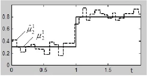
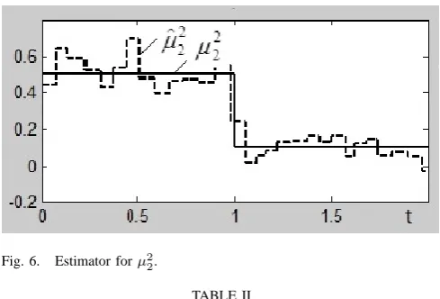
Fig. 3 – Fig. 6 demonstrate examples of the sequences of TAR(2)/ARCH(1) parameters estimates for H = 100. Here solid lines indicate true values of the parameters, and dotted lines shows the behavior of estimates. Every time unity corresponds to 10000 observations.
Further we conducted simulations of the proposed change point detection procedure. The simulations were conducted for the TAR(2)/ARCH(1) process. Before the instantθit was specified by the equation (1) with the parameters
Λ1= [ 0.5, 0.3 ], Λ2= [ 0.3, 0.5 ]; ω= 0.4, α= 0.1,
[image:13.595.301.540.163.400.2]Fig. 3. Estimator forµ11.
Fig. 4. Estimator forµ2 1.
After the instantθ= 10000he parameters are
Λ1= [ 0.2, 0.2 ], Λ2= [ 0.8, 0.1 ];
ω= 0.4, α2= 0.6,
[image:13.595.303.540.279.413.2]In this process in form (22) the noise variance is bounded from above by unity both before and after the change point. The change point θ= 10000 and δ= 0.025. Note that we choose the change point as a rather big number in order to have possibility to estimate the mean number of observation between false alarm using a sufficient sample size.
Fig. 5. Estimator forµ1 2.