The regression of a discrete dataset is a task which has to be solved if we need to obtain a mathematical model of the acquired data (Veselý 2011). The regres-sion will result into a mathematical function which approximates the dataset. As stated in (Meloun and Militký 1994), there are cases where the mathemati-cal model is known and the task is limited to finding the specific constants which suits the model best. A more difficult scenario is that we are not sure which mathematical model describes the dataset well and we need to find one and also to optimize its constant values. Such problem can be solved with the gram-matical evolution (Koza 1992; O’Neill et al. 2004).
In this contribution, we will describe and explain the solution of the regression problem using the grammatical evolution and differential evolution on the selected examples. We will present the advan-tages and results of such approach. For testing, we selected a textbook example from (Meloun 1996) of a regression used for the mental load dataset. Two variants of that example were used. The quality of solution is measured using the SSE (Sum of Squared Error) value.
Our target is to demonstrate the power of the two-phase grammatical evolution approach and to test whether this approach is capable to compete with the classical methods. A regression task can be completely automated by using this approach. Such automation can save expensive human resources.
MATERIAL AND METHODS
In this chapter, the testing data and used algorithms will be described. Also the settings for evolutionary process along with the grammar for chromosome translation will be disclosed.
The problem and data
As mentioned, two variants of one example were selected for the method testing. Both datasets are measurements of the mental load of an intensive brain activity of the test person from the textbook (Meloun 1996). The measurement contained values of the mental load measured over time with 1s step. In the source literature, a formula of the mathematical model was presented. The formula can be found as the equation (1). The variable x is the time measured in seconds.
y(x) = a + b × ec×x (1)
The two datasets were named CASY3 and CASY5. Figure Figure 1. The visualized CASY3 dataset (a) and CASY 5 dataset (b) contains the plots of both datasets. The vertical axis of plots is set to the in-terval of interest on purpose. We can observe that the beginning of both datasets has roughly constant
Automatic discovery of the regression model
by the means of grammatical and differential evolution
Jií LÝSEK, Jií ŠŤASTNÝ
Department of Informatics, Faculty of Business and Economics, Mendel University in Brno, Brno, Czech Republic
Abstract: In the contribution, there is discussed the usage of the method based on the grammatical and diff erential evolu-tion for the automatic discovery of regression models for discrete datasets. Th e combination of these two methods enables the process to fi nd the precise structure of the mathematical model and values for the model constants separately. Th e used method is described and tested on the selected regression examples. Th e results are reported and the obtained mathema-tical models are presented. Th e advantages of the selected approach are described and compared to the classical methods.
Key words: context-free grammar, evolutionary methods, genetic algorithm, sum of squared error
values and from the beginning of the experiment (which exact time is given in the task definition), the value starts to decrease. The presented formula is valid only for those decreasing parts of datasets. The constant part of the measurement was removed. The beginning of the dataset CASY3 is from ninth second and the beginning of the CASY5 dataset is from fifth second.
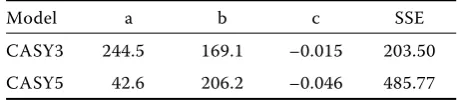
The values of constants a, b and c given in the problem definition are disclosed in Table 1. The constants of the problem model. The mathematical model quality is measured using the SSE value which is also presented in the same table.
Evolutionary methods
Evolutionary methods are the algorithms inspired by the evolution in living nature. Genetic algorithms, the grammatical evolution and the differential evolution are methods belonging into this algorithm category (Mitchell 1999). These optimisation algorithms are iterative and stochastic. At present, they are being used in various fields of research. Their largest ad-vantage of these methods is the capability to solve almost any difficult optimisation problem. They also can be adapted to solve many various problems such as planning (Alabdulkader et al. 2012; Čížek and
Šťastný 2013), learning (Škorpil and Šťastný 2009; Lýsek et al. 2012) and even the automatic creation of computer programs and many other applications (Koza 1992; Munk and Drlík 2011; Beránek 2012). On the other hand, these algorithms consume quite large computing resources.
New areas of research can benefit from the usage of such algorithms as the computing power increases significantly in the years. These algorithms substan-tially benefit from the ability of new processing units to perform computations in parallel.
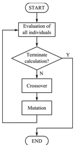
The evolutionary algorithm uses operators inspired by nature such as the crossover and mutation to explore new solutions of the given problem. The crossover operation is responsible for the recombi-nation of the existing individuals into new ones. The capability of the algorithm to search for solutions which are not combinations of the initial population is provided by the mutation operator. This operation randomly modifies the selected individuals.
Each iterative run of the algorithm consists of the evaluation of all members in the population; the in-dividuals are selected for the crossover based on their quality (calculated by the capability to solve the given problem). The better the individual performance, the higher is its chance to reproduce. The resulting members are used to compose a new population. The flow of the algorithm is shown in Figure 2. The flow of the genetic algorithm.
The whole process is driven by the fitness function, which is a formula that measures the quality of each individual in the population. Based on the fitness value, the individual is selected for the crossover more or less often.
Each individual contains the genetic information stored in the chromosome which is presented as the 320
340 360 380 400
[image:2.595.98.531.82.235.2]1 4 7 10 13 16 19 22 25 28 31 34 37 40 43 46 CASY3 dataset
Figure 1. The visualized CASY3 (a) and CASY 5 (b) dataset
[image:2.595.60.289.691.742.2]Source: Meloun (1996)
Table 1. The constants of the problem model
Model a b c SSE
CASY3 244.5 169.1 –0.015 203.50
CASY5 42.6 206.2 –0.046 485.77
Source: Meloun (1996)
one-dimensional array of numbers. The values of the chromosome represent the solution of the given problem in some form. The chromosome encoding can be different for every problem being solved. To calculate the fitness value, the chromosome has to be decoded and the individual has to be evaluated.
First phase of the regression model search – the grammatical evolution (GE)
We used the grammatical evolution (Ryan and O’Neill 2003) with the backwards processing of the chromosome (Popelka and Šťastný 2009). The framework is our own system written in the Java programming language. The system was also used in our previous research published in (Lýsek et al. 2012; 2013).
The grammatical evolution combines the evolu-tionary methods with the context-free grammars (Hopcroft and Ullman 1969). The grammar is defined by a set G = {N, T, P, S}. N is a set of non-terminal symbols. T is the set of terminal symbols (the result-ing computer program is composed of these). P is the of production rules which are used to translate the non-terminals into terminals. The starting symbol is denoted S. This approach is inspired by the genetic programming (Koza 1992).
The values of the chromosome are used to select the variant of the production rule. If the chromo-some contains for example value 20 and we should translate the non-terminal with 6 possible rewrites, we calculate the modulus of division 20 mod 6 = 2 and therefore we select the third possible rewrite. The indexing has to be zero based.
The length of the chromosome is given and it defines the maximal length and complexity of the resulting regression model. We employed a custom operator to maintain the diversity of the population by calculating the Levenshtein distance (Levenshtein 1966), of string representations of the population members. The diversity operator function descrip-tion follows:
– Take the current population of individuals ordered by their quality (the best individuals are on top) as an input.
– Create the temporary population.
– Pick all members of this population one by one. – Pick each member of the temporary population
and compare the string distance. Remember the lowest value.
– If the distance between any two individuals is smaller than a certain threshold value, do not add the member of the input population into the temporary population, otherwise, the member is added into the temporary popula-tion.
– Fill the temporary population with random indi-viduals up to the specified capacity.
– Return the temporary population as an output.
Second phase of the regression model search – the differential evolution (DE)
To achieve the best result, we introduced second phase of optimisation. This phase is based on the differential evolution algorithm (Price et al. 2005). Second phase is executed if the translated individual contains one or more constant terminal nodes. This terminal has a default value set to zero, but this value can be adjusted by the differential evolution. There is a possibility to use another optimisation algorithm but we choose to implement the algorithm based on the evolution as we were able to use the common programming technique.
The differential evolution is a process designed for the optimisation of numeric values. The length of the chromosome is variable and in our approach it is determined by the amount of constant nodes.
[image:3.595.109.239.81.333.2] Figure 2. The flow of the genetic algorithmThe crossover and mutation operations are replaced by one reproduction procedure. The simplified re-production procedure description follows:
– Select three different members’ mj, mk and ml for each member mi in the current population. The members must be different so that i ≠ j ≠ k ≠ l.
– Create the temporary chromosome chtemp which gene values are calculated by formula 2. The value
MR is the mutation rate.
– The chromosome of the selected individual chi and chromosome chtemp are combined randomly based on the value of the crossover probability.
݄ܿ௧ൌ ݄ܿ ܯܴ ൈ ሺ݄ܿെ ݄ܿሻ (2)
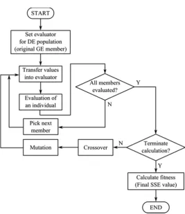
The procedure of the constant optimisation is in Figure Figure 3. The flow of the differential evolu-tion for the constant optimisaevolu-tion. The described DE process is executed optionally before each fitness calculation in the GE process. The condition is based on the presence of constant terminals in the translated individuals. As the fitness evaluator for each member of the DE process is set the original GE member. In every iteration of the differential evolution algorithm, the optimised constant values of each DE member are transferred into the GE member in sequence. The fitness value is calculated for all DE members in the current population using the GE program with
the assigned constants. The resulting fitness value is stored into the DE member.
Parameters of the genetic algorithm and experiment settings
[image:4.595.64.332.74.384.2]The parameters with most significant effect on the evolutionary process are presented in this section for both the grammatical and differential evolution. Table 2 contains the overview of these parameters. As a selection strategy, there was used the
Figure 3. The flow of the differential evolu-tion for the constant optimisaevolu-tion
[image:4.595.306.532.597.742.2]Source: Popelka and Šťastný (2009)
Table 2. The parameters of the GE and DE algorithms
GE phase DE phase
Population size 2000 20
Iteration count 500 50
Chromosome length 20 Variable
Crossover rate 0.8 0.5
Mutation rate 0.1 0.5
Elitism Off Off
Selection strategy Tournament selection/5 Tournament selection/5
ment selection of size 5 for both processes (Miller and Goldberg 1995).
Also the fitness formula is very important as it guides the optimisation process towards the requested results. We used the SSE value directly as a fitness value for both optimisation phases. The formula used for the calculation of the fitness value F for the individual m follows:
ܨሺ݉ሻ ൌ ሺݕௗെ ݕௗ௧ሻଶ
ୀଵ
(3)
The dataset contains n values; these are treated as control points yi data. The output values yi model
of the current model presented by the translated chromosome are subtracted from the control points. The results of subtractions are squared and added together. The lower the fitness value, the better is the individual.
This means that the strategy of the evolutionary algorithm is set to minimize the fitness value; such strategy forbids the usage of the popular roulette-wheel selection, but the used tournament selection is not affected. This kind of selection only requires information which of two compared individuals is better.
The procedure was executed multiple times (10 executions for the CASY3 dataset search and 20 executions for the CASY5 dataset search). The best individuals of all runs for each dataset will be pre-sented the results section.
The grammar used for the chromosome translation
The grammar we used contains only the termi-nal symbols, which we suppose the problem solu-tion will require. An attensolu-tion is required only for the terminals pdiv a plog. These two terminals are the modified mathematical operations division and natural logarithm. The first is modified such that the division by zero results into zero and not error. The latter returns also zero for the negative input values and zero. The reason of such modification is that we would like to preserve the mathematical model as it can possess a good structure and it can be later modified by hand.
<expr> ::= <var> | <const> | <math_op>
(<expr>,<expr>) | <math_fun>(<expr>) <math_op> ::= add | sub | mul | pdiv
<math_fun> ::= sin | plog | exp <const> ::= C
RESULTS AND DISCUSSION
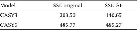
To measure the quality and to compare the mod-els, we calculated the SSE values for all four models (original models for the CASY3 and the CASY5 given by formula 1, the GE models for the CASY3 and the CASY5 created by our system). The resulting values were compared together. These calculations were done in the Matlab environment.
Table 3 contains the comparison of the models qual-ity. The quality of both our models is better than the quality of the source models. For the CASY3 dataset, the difference is quite high. Our CASY5 model is, on the other hand, only very slightly better.
Regression models created by our algorithm are presented here. Constant values are inserted directly into the model, as that is the form of output from our framework. The CASY3 dataset model follows: sub(394.2327778621829,sub(plog(3897.3005844181 68),sub(mul(sin(plog(x)),19.024858864988794),x)))
And regression model for CASY5 dataset: add(mul(103.37341027736862,sin(plog(x))),sub(sub (x,cos(5110.130972253164)),-474.6369460444114))
The resulting models can be optimized by hand – there are mathematical functions with constant param-eters which can be replaced by another constant. This post-processing function can also be implemented into the used framework.
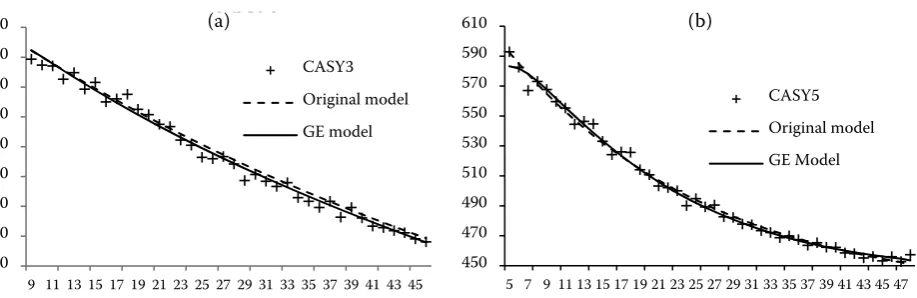
Finally in Figure Figure 4. Comparison of the GE and the original model for the CASY3 (a) and CASY5 (b) datasets Source: own data, there is a visual comparison of models for the CASY3 and CASY5 datasets. Our new models are presented as a continuous line, the original models have a dashed line. Crosses are the original data-points.
Two testing datasets (Meloun 1996) were used to demonstrate the ability of the evolutionary methods to solve the regression problem. The resulting model quality was measured using the SSE value which is a common measure of quality used in many regression or forecasting applications (Štencl et al. 2011). In one of the testing instances, we obtained the result better than the original model. In the second instance, the result was only slightly better. However, it is
pos-Table 3 The comparison of the SSE values
Model SSE original SSE GE
CASY3 203.50 140.65
CASY5 485.77 485.27
[image:5.595.304.531.691.741.2]sible to obtain a better result in another run as the algorithm is stochastic.
Th e advantage of a better regression model is that the consequent calculations based on the regression model can gain more accuracy and less uncertainty (Popelka and Šťastný 2009; Kapounek and Poměnková 2013).
CONCLUSION
In this contribution, we demonstrated the usage of the two-phase evolutionary approach used for the model search. This approach can help to create more accurate regression models in any field of research.
The main advantage of this approach is that the method is capable to find the model automatically without any need to specify even the rough structure of it. This ability can be utilized when the methods are not applicable – the character of the dataset is, for instance, impossible to approximate by a single mathematical function.
Another advantage is the division of the process into two separate phases. The first phase is a search for the optimal model structure; this is accomplished by the grammatical evolution method. The second phase is the optimisation of the model constants; we used the differential evolution method for this task. In the future research, we would like to test other optimisation methods, suitable for the numerical values optimisation, for this phase. The differential evolution method may be used separately to improve the existing regression models.
Moreover, our contribution proves that even if the character of the dataset is fairly simple, our combined method is capable of finding better results than the proposed mathematical model designed by hand. On
the other hand, the obtained mathematical model can be more difficult to understand and can be more complex. The structure of the model is not a problem if a computer is used to analyse the results.
Acknowledgement
This work has been supported by the grants: FSI-S-14-2533 Aplikovaná informatika a řízení – Research design of Brno University of Technology 2014 and IGA 6/2014 – Research design of Mendel University in Brno.
REFERENCES
Alabdulkader A.M., Al-Amoud A.I., Awad F.S. (2012): Optimization of the cropping pattern in Saudi Arabia using a mathematical programming sector model. Ag-ricultural Economics – Czech, 58: 56–60.
Beránek L. (2012): The Use of the Belief Function Theory for a Situation Inference. In: Proceedings of 18th
Inter-national Conference on Soft Computing – MENDEL, pp. 106–111. Brno University of Technology, Brno; ISBN 978-80-214-4540-6.
Čížek L., Šťastný J. (2013): Comparison of Genetic Algo-rithm and Graph-Based AlgoAlgo-rithm for the TSP. In: 19th
International Conference on Soft Computing – MENDEL 2013. Brno University of Technology, Brno, pp. 433–438; ISBN 978-80-214-4755-4.
Hopcroft J.E., Ullman J.D. (1969): Formal Languages and their Relation to Automata. Addison-Wesley, Boston; ISBN 978-0201029833.
Kapounek S., Poměnková J. (2013): The endogeneity of optimum currency area criteria in the context of finan-320
330 340 350 360 370 380 390 400
9 11 13 15 17 19 21 23 25 27 29 31 33 35 37 39 41 43 45 CASY3
CASY3 Original model GE model
450 470 490 510 530 550 570 590 610
5 7 9 11 13 15 17 19 21 23 25 27 29 31 33 35 37 39 41 43 45 47
[image:6.595.74.533.79.228.2]CASY5 Original model GE Model
Figure 4. Comparison of the GE and the original model for the CASY3 (a) and CASY5 (b) datasets
Source: own data
cial crisis: Evidence from the time-frequency domain analysis. Agricultural Economics – Czech, 59: 389–395. Koza R.J. (1992): Genetic Programming II: On the
Program-ming of Computers by Means of Natural Selection. The MIT Press; ISBN 0-262-11170-5.
Levenshtein V.I. (1966): Binary codes capable of correct-ing deletions, insertions, and reversals. Soviet Physics Doklady, 10: 707–710.
Lýsek J., Šťastný J., Motyčka A. (2012): Object Recognition by means of Evolved Detector and Classifier Program. In: Proceedings of 18th International Conference on Soft
Computing – MENDEL 2012, pp. 82–87. Brno University of Technology, Brno; ISBN 978-80-214-4540-6. Lýsek J., Šťastný J., Motyčka A. (2013): Comparison of
Neural Network and Grammatical Evolution for Time Series Prediction. In: Proceedings of 19th
Internation-al Conference on Soft Computing – MENDEL 2013, pp. 215–220. Brno University of Technology, Brno; ISBN 978-80-214-4755-4.
Meloun M., Militký J. (1994): Statistické zpracování ex-perimentálních dat v chemometrii, biometrii, eko-nometrii a v dalších oborech přírodních, technických a společenských věd. (Statistical processing of experi-mental data in chemometry, biometry, econometry and in other fields of natural and social sciences.) Plus Praha. ISBN 80-85.
Meloun M. (1996): Statistické zpracování experimentálních dat: sbírka úloh. (Statistical processing of experimental data: workbook.) Univerzita Pardubice; ISBN 80-7194-075-5.
Miller B.L., Goldberg D.E. (1995): Genetic Algorithms, Tournament Selection and the Effects of Noise. IlliGAL Report No. 95006, Department of General Engineering, University of Illinois, p. 13.
Mitchell M. (1999): An Introduction to Genetic Algo-rithms. MIT Press, Cambridge, Massachusetts; ISBN 0−262−13316−4.
Munk M., Drlík M. (2011): Influence of different session timeouts thresholds on results of sequence rule analysis in educational data mining. Communications in Com-puter and Information Science, 166: 60–74.
O’Neill M., Brabazon A., Adley C. (2004): Automatic Gen-eration of programs for Classifcation Problems with Grammatical Swarm. In: Proceedings of the 2004 IEEE Congress on Evolutionary Computation (CEC 2004), pp. 104–110. Portland, Oregon; ISBN 0-7803-8515-2. Popelka O., Šťastný J. (2009): WWW portal usage analysis
using genetic algorithms. Acta Universitatis Agriculturae et Silviculturae Mendelianae Brunensis, 6: 201–208. Popelka O., Šťastný J. (2009): Uplatnění metod umělé
inteli-gence v zemědělsko-ekonomických predikčních úlohách. (Using artificial intelligence methods for agricultural and economic data prediction.) Folia Universitatis Ag-riculturae et Silviculturae Mendelianae Brunensis, Brno; ISBN 978-80-7375-340-5.
Price K.V., Storn R.M., Lampinen J.A. (2005): Differential Evolution – a Practical Approach to Global Optimiza-tion. NCS Springer, Berlin Heidelberg; ISBN 978-3-540-31306-9.
Ryan C., O’Neill M. (2003): Grammatical Evolution: Evo-lutionary Automatic Programming in an Arbitrary Language. Kluwer Academic Publishers; ISBN 978-1-4615-0447-4.
Škorpil V., Šťastný J. (2009): Comparison Methods for Object Recognition. In: Proceedings of the 13th WSEAS
International Conference on Systems. Rhodos, Greece, pp. 607–610; ISBN 978-960-474-097-0.
Štencl M., Popelka O., Šťastný J. (2011): Comparison of time series forecasting with artificial neural network and statisticial approach. Acta Universitatis Agriculturae et Silviculturae Mendelianae Brunensis, 2: 347–352. Šťastný J., Škorpil V. (2007): Genetic Algorithm and Neural
Network. In: Proceedings of the 7th WSEAS International
Conference on Applied Informatics and Communica-tions, Vouliagmeni, Greece, pp. 347–351. ISSN 1790-5117. ISBN 978-960-8457-96-6.
Veselý A. (2011): Economic classification and regression problems and neural networks. Agricultural Econom-ics – Czech, 57: 150–157.
Received: 25th August 2014
Accepted: 27th September 2014
Contact address:
Jiří Šťastný, Department of Informatics, Faculty of Business and Economics, Mendel University in Brno, Zemědělská 1, 613 Brno, Czech Republic