A Life Cycle on Processing Large Dataset - LCPL
Rajit Nair
MANIT, Bhopal
Amit Bhagat,
PhD
MANIT, Bhopal
ABSTRACT
We all know that today’s era is of big data, we can also call it as large data set where data from different sources are collected at one place and it is very difficult to process these type of data. Mainly these types of data are collected where there is huge volume, high velocity and different varieties of data. These types of data are processed for analytical purpose because if we did not analyze it then there is no sense of collecting these type of data. So in this paper we are explaining about the life cycle of processing large data set and propose a new term for it i.e. LCPLD(Life Cycle on Processing Large Data set. Here the discussion will mainly focus on the steps which are involved during the life cycle of processing that are pre-processing, feature selection, feature extraction, classification, clustering and many more.
General Terms
This survey paper is basically used to represent the life cycle of the processing of large data set. Mainly it emphasize on the overall processing of Big data or high dimensional data.
Keywords
Preprocessing Features, Classification, Clustering, Dimensions, Features.
1.
INTRODUCTION
We wrote this paper because the only reason is that, we face many problems during the research in the area of big data and we don’t know from where we have to start and what would be our approach. So mainly this paper tell us that what are the steps involved in the big data [1] processing for the analysis purpose. In this paper we will discuss the main three steps involved in big data processing [2]. These steps are pre-processing which also include feature selection or feature extraction and the last one is classification and clustering. In pre-processing step we will discuss why the data is processed and what the need of it. In feature selection or feature extraction [3] we will discuss why large data set is reduced to small data set after preprocessing, but we must be aware of that feature selection [4] and feature extraction is also a part of preprocessing, we termed it separately just for the explanation purpose. This step is done because it is very difficult to analyse large data set so it is much needed that it must be reduced to small data set without any loss of information. Now the last step is classification [5] & clustering [6], this is also one of the major step because without this step we cannot say in what category our data belongs. Classification is done mainly for supervised learning and clustering is mainly done where we are dealing in unsupervised way. We will discuss all the steps in detail in the further sections. Our further section will be stated as follows (i) Data Preprocessing (ii) Feature selection & Feature extraction (iii) Classification & Clustering.
2.
DATA PRE-PROCESSING
Large data set come from heterogeneous or many different sources have many different attributes. Many times we call it
as high dimensional data [7], here dimension means attribute. Therefore, many software tools are required for exploratory analysis and development of analytics. Tools must be also capable of accessing the data from different sources and form the dataset for the analysis purpose. We all must be aware that these real world data are incomplete, noisy and inconsistent. So data preprocessing is very important procedure for processing as well as for the analysis also.
2.1
What is the need of Data
Pre-processing?
Preprocessing is needed always when we are performing any big task because it is the preparation taken before actual processing, same way in case of data preprocessing when we are dealing with big amount of information, this process cleans and prepares the data for further analysis purpose. If it is not done in that case there is possibility that we might deal with wrong or incorrect data and this incorrect data may lead us to inaccurate or misleading result which will impact our performance as well as the reliability of the predictive model [1]. Our main goal is to find out the most predictive features of the data, so that we can enhance the power of the analytics model.
In this whole process we collect the data that has been collected from data pre-processing is taken and implemented across a number of analytics-driven systems. An example of this is the innovation to make cars smarter, even in many places it is used as exit poll results of election of the governing body. By using big data analytics [2] the place where enormous amounts of data are collected from real-world driving situations, recording data such as engine performance, video, radar, and other signals. This data is used to generate important metrics such as fuel economy and performance at the fleet level. Engineering teams are also using this real-world data to design, develop and test new types of automotive systems, such as advanced driver assistance systems (ADAS).
2.2
Techniques used for Data
Preprocessing
Fig 1: Different stages of data preprocessing [3]
This wider adoption of data preprocessing techniques is resulting in adaptations of known models for related frameworks or completely novel proposals. Now we will discuss how we will deal with imperfect and imbalanced data.
2.3
Data Cleaning
It can be first process of data preprocessing, because for analysis we always need the data which is clean and our real world data is far from clean data. Cleaning mainly consist of two stages i.e. error detection [3] and error repairing. Crowdsourcing [4] is one of the approaches or techniques which is widely used in Machine Learning to improve accuracy or efficiency. During the process we must focus on deduplication (Duplication Error), repairing missing and incorrect values (Attribute Error), and the removal of erroneous or irrelevant data. To overcome from these errors the operations done are mainly value imputation data repairing, entity resolution, error/outlier removal respectively
.
2.4
Data Transformation
This method converts our big data into some meaningful information elements that is incorporated into business intelligence and predictive analytics. The transformation process includes many data manipulations such as moving, spitting, translating, merging, sorting, pivoting and many more. For e.g. we have seen many time times that our name is split into two names like first name and last name another one is when our dates are changed to prescribed format even if we given in any format. Often this step also involves validating the data against data quality rules.
2.5
Missing Values imputation
In analytics we assume that our large data set is complete, but it is very common that there may be presence of missing values. Because of faulty sampling process we cannot store or collect missing values. We cannot ignore missing values because in data analysis it may create very difficult problem for the analyst. It is not a easy task to handle the missing data, if we handle it appropriately it may lead to incorrect analysis. Due to this performance can be degraded. There are many ways to handle this problem, but we will not discuss all the methods. The very first method is to ignore those instance which contain a missing value, as we have seen it is not very beneficial because it may possible the instance which you are
avoiding or discarding may contain useful information, so if it is discarded this may lead to bad analysis.
Another way to handle missing values is to works on data derive from statistics. In this method the probability function is taken into account which can generate the desired missing value. Most of the time we use likelihood procedure, they may create probabilistic models which can fill missing values. The probability model for most of the dataset is usually unknown, so to handle these dataset we use machine learning techniques because machine learning concept is mostly where we don’t have any prior information regarding the target variable.
2.6
Data Integration
Data integrations is the another major step in data pre-processing, integration is needed because the data which is collected that comes from the different sources and we have to combine this data from analysis. We must have to find ways which can manage these terabytes or petabytes of data in a way that can generate good analysis result. This must be easy, fast and affordable. A tightly coupled data integration and data analytics platform accelerates the realization of value from blended big data. The points which considered in the data integration are as follows:
• Full array of analytics: data access and integration to data visualization and predictive analytics.
• Empowers users to architect big data blends at the source and stream them directly for more complete and accurate analytics.
• Ability to spot check data in-flight with immediate access to analytics, including charts, visualizations, and reporting, from any step in data preparation.
• Supports the broadest spectrum of big data sources, taking advantage of the specific and unique capabilities of each technology.
• Open, standards based architecture makes it easy to integrate with or extend existing infrastructure.
2.7
Noise treatment
It is already discussed in the above section that the actual data is rarely perfect and we know that the quality of analysis depend on the quality of data. So another important aspect of pre-processing is noise removal, a noise is nothing it is the unwanted data which does not make any impact on our analysis, it can affect the input feature features or output features or sometimes both. The two main types of noise are attribute noise and class noise. The attribute noises are those which occur in the input attributes. When the noise affects the output attribute that is the worst condition and this kind of noise can be seen during the classification process.
instead of discarding they are repaired. In case of repair they replace the corrupted values with some more appropriate values. After this the corrected values are injected into the data set.
But all the three methods have their own advantages and disadvantages and this totally depend on the size and characteristic of the data set.
2.8
Data Normalization
In big data world, not all data is formatted in our desired format. This paragraph will show you how to normalize and discretize data. If the data is noisy and in order to handle the noisy data, we must transform them globally, this can be done in two ways. First one is to reduce the grain in the data, it's called discretize, from fine grain to higher grain. For example, from numeric to nominal. And the other main way is to change the scale or range as the data, it's called normalize. It might also be necessary to discretize to apply different data analytics models and methods because some prediction methods require a nominal attribute instead of a numeric continuous attribute. So let's first see how to normalize data. Normalization consists in changing the scale in the data, when you have data of mixed scale. For example, you may have mixed data from different data sources. We've talked about merging key con data with gene expression data in the same dataset. In this case, you're going to have data of mixed scales. And so for data analytics methods, journeys don’t behave very well with different scales, and you want to deal with that. For example, age and income may have widely different ranges. It is frequent to scale all data between the ranges -1, 1 or 0, 1. So all data values will be within these scales. And to accomplish that you normalize your data. Generally, data are scaled into a smaller range. Example, we have age values that say between 0 and 150, to be sure to include everyone. And you want to normalize it int 0,1. Intuitively, you see that someone of age 50 is around 0,150 is about one-third of the range. So intuitively, you can say if I map that into a range 0, 1, the age of this person will be 0.33. A lot of statistical methods, they have some requirements about the shape in your data and they perform better so data is normalized.
3.
DIMENSIONALITY REDUCTION
-FEATURE SELECTION & -FEATURE
EXTRACTION
As we must remember the strategies which has been discussed above are also a partial process of dimensionality reduction, but here will explain separately about the dimensionality reduction techniques and we will also discuss some of the methods which has not been discussed in the above section, which are also process in dimensionality reduction. Before discussing dimensionality reduction we must know what is dimension, dimensions can be defined as the set of attributes or features which are in the data set, if it is large data set or big data set then it can be called as high dimensional data set. It is very difficult to process or analyze this high dimensional data, so dimensional reduction techniques are the ways by which we can convert a high dimensional data into low or lesser dimensions, but we must always consider that information must not be lost otherwise dimensional reduction does not make any sense. These techniques are very crucial in the area of big data analytics because by this we can obtain better features for analysis.
Let’s look at the image shown below. It shows 2 dimensions x1 and x2, which are let us say measurements of several object in cm (x1) and inches (x2). Now, if you were to use
[image:3.595.322.532.129.260.2]both these dimensions in machine learning, they will convey similar information and introduce a lot of noise in system, so you are better of just using one dimension. Here we have converted the dimension of data from 2D (from x1 and x2) to 1D (z1), which has made the data relatively easier to explain.
Fig 2: Representation of two dimensional features [4]
In similar ways, we can reduce n dimensions of data set to k dimensions (k < n). These k dimensions can be directly identified (filtered) or can be a combination of dimensions (weighted averages of dimensions) or new dimension(s) that represent existing multiple dimensions well. One of the most common application of this technique is Image processing. You might have come across this Facebook application – “Which Celebrity Do You Look Like?”But, have you ever thought about the algorithm used behind this?
3.1
Benefits of Dimension Reduction
Let’s look at the benefits of applying Dimension Reduction process:
• It helps in data compressing and reducing the storage space required.
• It fastens the time required for performing same computations. Less dimensions leads to less computing, also less dimensions can allow usage of algorithms unfit for a large number of dimensions.
• It takes care of multi-collinearity that improves the model performance. It removes redundant features. For example: there is no point in storing a value in two different units (meters and inches).
• Reducing the dimensions of data to 2D or 3D may allow us to plot and visualize it precisely. You can then observe patterns more clearly. Below you can see that, how a 3D data is converted into 2D. First it has identified the 2D plane then represented the points on these two new axis z1 and z2. • It is helpful in noise removal also and as result of that we can improve the performance of models.
Fig 3: Transformation from 3 dimensional to 2 dimensional
[image:3.595.317.540.629.725.2]3.2
Feature Selection
First we must know what is feature? Feature is an attribute or variable and in case of high dimensional or big dataset there will be large number of features or variables. If we include all the features or variables during processing then it will be very tedious task and it will not make sense, so it is better we must select the feature or variable. Variable selection is an important aspect of model building which every analyst must learn. We must also consider one thing during feature selection that there must not be any type of information loss. Due to this we get the model which if free from correlated variables, unwanted noise etc. However many analyst believe that keeping all the features or variables will provide good result, but it is not true because in dataset many features are there which does not make any sense, so processing these features will unnecessarily consume your time. Many times you will feel that discarding a feature from the dataset has increase the accuracy of the model.
It requires a lot of practice and efforts to select a proper feature and fits into a model. Some of the key features of feature selection are as follows:
Processing time will be decreased
Helps to train machine learning algorithm faster
Over fitting will be reduced
Interpretation of models becomes easy because complexity also get easy after applying feature selection.
Feature selection has several advantages [1], such as:
Improving the performance of the machine learning algorithm.
Data understanding, gaining knowledge about the process and perhaps helping to visualize it.
Data reduction, limiting storage requirements and perhaps helping in reducing costs.
Simplicity, possibility of using simpler models and gaining speed.
Now we will discuss the methods for feature selection which are as follows:
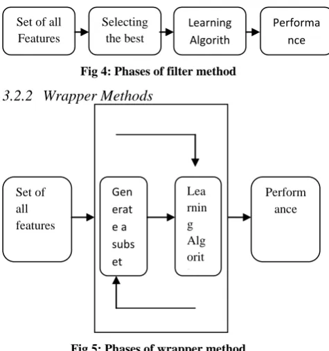
1. Filter Methods
2. Wrapper Methods
3. Embedded Methods
3.2.1
Filter Methods
It is one of the easiest method for applying feature selection. It did not depend on any machine learning algorithms. Features are selected on the basis of various statistical measures score and it is independent of any predictor and totally depends on the characteristic of training set on the basis of which selects the features. To select the features statistical methods are used like chi square method, r square method and many more. These are usually computationally less expensive than other existing methods like wrapper, embedded etc. It does not give better result for large dataset.
Mostly in case of this method we try to find correlation between features, on the basis of which we can select or discard the features. Correlation gives you idea that how much the features are similar to each other. For an example if two features are very much correlated with each other in that case we can discard any one of them. Features and response can be
[image:4.595.317.537.106.172.2]continuous or categorical, a table 1. is given below which shows methods which we can apply depending on the dataset. Table 1. Types of features
Feature\Response Continuous Categorical
Continuous Pearson’s Correlation
LDA
Categorical Anova Chi-Sqaure
Brief explanations about these methods are as follows: • Pearson’s Correlation: It is used as a measure for quantifying linear dependence between two continuous variables X and Y. Its value varies from -1 to +1. Pearson’s correlation is given as
:
𝜌 𝑋, 𝑌 = 𝑐𝑜𝑣 (𝑋,𝑌)𝜎
𝑋𝜎𝑌
• LDA: Linear Discriminant Analysis is used to find a linear combination of features that characterizes or separates two or more classes (or levels) of a categorical variable.
• ANOVA: ANOVA stands for Analysis of variance. It is similar to LDA except for the fact that it is operated using one or more categorical independent features and one continuous dependent feature. It provides a statistical test of whether the means of several groups are equal or not.
[image:4.595.314.552.420.674.2]• Chi-Square: It is a statistical test applied to the groups of categorical features to evaluate the likelihood of correlation or association between them using their frequency distribution. Filter methods never deal with multicollinearity, so we must deal with it before training models of the data.
Fig 4: Phases of filter method
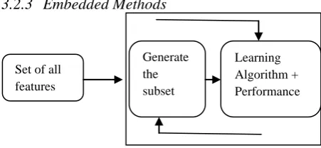
3.2.2
Wrapper Methods
Fig 5: Phases of wrapper method
In contrary to feature selection method, wrapper method use predictor during the whole process. It is more expensive than filter method, used for large data set but give better results.. Here we try to use a subset of features by which we train a model. On the basis of previous result it decides whether we have to select or discard the features. This problem is reduced to search problem. The approaches we follow in this method
Set of all features
Perform ance
Gen erat e a subs et
a subs et
a subs et
Lea rnin g Alg orit hm Set of all
Features
Selecting the best
subset
Learning Algorith
m
are mainly forward, backward, recursive feature elimination methods.
Forward Selection: It is the simplest greedy search algorithm and an iterative approach in which we don’t have any feature at the starting, after each iteration they keep adding the unused feature which suits the best for our model. For each addition performance is estimated using the cross validation. Feature having the highest performance will be considered for the objective function. After that new round will be started with modified selection. This way it selects features from the dataset.
Backward Elimination: As name already suggest that this will be the reverse process of forward feature selection process, in which we start with considering all features after that each attribute will be removed on every iteration, after removing feature we will calculate the performance using the cross validation. The attributes giving less performance will be removed from the process. The removal can be done in two steps firstly it can discard several features and secondly it permit us for backtracking. In this method it may happen that after removal of many features its performance will be degrade, in that case we must add those eliminated feature due to which performance has been degraded. Again we have to do revaluation for the new subset of the process.
Recursive Feature elimination: It is slightly different from other two approaches which we discussed above, It is also greedy based algorithm, which targets the subset with best performance. It creates the model recursively and kept the best and the worst performing feature aside after each iteration. It develop the next one with the remaining features and do this process until all the features get exhausted. Then it ranks the features based on the order of their removal. Let us discuss an practical approach for implementing feature selection, the implementation can be done in any language like python, R, Matlab etc., Here we will use Boruta package in python that finds the importance of a feature by creating shadow features. Steps are as follows:
Firstly, it adds randomness to the given data set by creating shuffled copies of all features (which are called shadow features).
Then, it trains a random forest classifier on the extended data set and applies a feature importance measure (the default is Mean Decrease Accuracy) to evaluate the importance of each feature where higher means more important.
At each iteration, it checks whether a real feature has a higher importance than the best of its shadow features (i.e. whether the feature has a higher score than the maximum Z-score of its shadow features) and constantly removes features which are deemed highly unimportant.
Finally, the algorithm stops either when all features get confirmed or rejected or it reaches a specified limit of random forest runs.
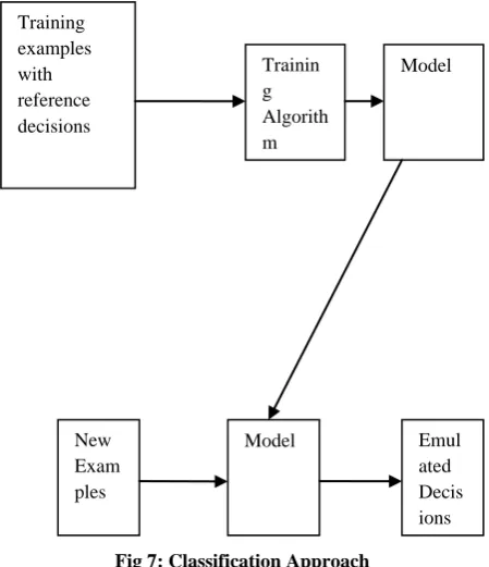
[image:5.595.53.279.648.752.2]3.2.3
Embedded Methods
Fig 6: Phases of Embedded method
This method have quality of both filter and wrapper methods. Embedded methods combine the qualities of filter and wrapper methods. There is no theoretical frame work which has been developed to embedded methods. This method differ from filter and wrapper method in the way feature selection and learning algorithm interact, here learning part and the feature selection part cannot be separated. Filter method do not incorporate training and wrapper methods use machine learning to measure the performance of the subset of features without embedding any knowledge about the specific structure of the classification or regression. The algorithms which implement this have their own inbuilt feature selection methods. There are many examples based on this method like LASSO regression, RIDGE regression and many more.
Lasso regression performs L1 regularization which adds penalty equivalent to absolute value of the magnitude of coefficients.
Ridge regression performs L2 regularization which adds penalty equivalent to square of the magnitude of coefficients. Difference between Filter and Wrapper methods
The main differences between the filter and wrapper methods for feature selection are:
Filter methods measure the relevance of features by their correlation with dependent variable while wrapper methods measure the usefulness of a subset of feature by actually training a model on it.
Filter methods are much faster compared to wrapper methods as they do not involve training the models. On the other hand, wrapper methods are computationally very expensive as well.
Filter methods use statistical methods for evaluation of a subset of features while wrapper methods use cross validation.
Filter methods might fail to find the best subset of features in many occasions but wrapper methods can always provide the best subset of features.
Using the subset of features from the wrapper methods make the model more prone to over fitting as compared to using subset of features from the filter methods.
Out of the above three methods we cannot say which one is the best method, it totally depends on the dataset and the application. Filter performs faster in small dataset but it is not got for large dataset.
3.3
Feature Extraction
Feature extraction is the way of dimensional reduction or extracting the feature. It performs transformation by which it generate other features or subset which are more significant or we can say it is a way by high dimensional data is transformed to low dimensional space.. "Feature extraction is generally used to mean the construction of linear combinations αTx of continuous features which have good discriminatory power between classes". It is used to reduce complexity and give a simple representation of data representing each variable in feature space as a linear combination of original input variable. The most popular and widely used feature extraction approach is Principle Component Analysis (PCA) introduced by Karl. It is important that for subsequent analysis of pattern recognition, visualization or anything else that the data must be represented in a manner that facilitates the analysis. Feature extraction methods found much more suitable for automated detection of ophthalmologists diseases than feature Set of all
features
Generate the subset
selection methods because of noisy data. Because most of the datasets related to bio medical contain noisy data instead of irrelevant or redundant data. In statistical learning, the process of identifying the meta variables is known as feature extraction. Some of the methods of feature extraction are as follows:
Data descriptive Statistics
This mainly shows the basic feature of the data in the study, if we consider sensors in that case data description will be shown by RMS, correlation coefficient, variance, crest factor kurtosis etc. Other than sensor if we take event into account in that case data description will be shown by count, duration time, occurrence rates, delays etc.
Data descriptive models
This model basically helps us to understand the behavior. We can build any type of model that totally depends on the task or application. The models can be distributive, Information-based, regression, classification or clustering based. The distributed models can be shown by Histogram, parametric distribution etc. Information based can be implemented by mutual information, minimum descriptive length etc. Regression by curve fitting, AR models etc.
Time-independent transforms
This can be done by mathematical operation like difference, logarithm, summation ratio etc. This transformation can also done by principal component analysis independent component analysis etc.
Feature extraction is classified into two categories linear & non-linear methods. Explanation of these method are as follows:
3.3.1
Linear Methods
As we know feature extraction is the most important issue in pattern recognition. Its main focus is on finding linear transformation, which map the original high dimensional space into low dimensional space but that must contain all the explanatory information. Linear methods are mostly used as preprocessor before applying complex non linear classifiers. Many methods are there but the two most common methods based on linear methods are PCA and ICA.
3.3.2
Non linear methods
Sometimes linear methods are not capable to do classification of linearly non-separable classes. Thus kernel methods have been proposed to overcome this limitation. Firstly this method transforms the data samples into higher dimensional space via non linear mapping and then applies the linear methods in this space. However, in most cases we may not have sufficient prior knowledge to design or the mapping of the data samples into a higher-dimensional space explicitly cannot be intractable. In such cases, we utilize kernel functions to overcome these limitations. Some of the popular non linear methods are Non Linear Principal Component Analysis (NPCA) or Kernel Principal Component Analysis (KPCA), Non Linear Discriminant Analysis (NLDA), Kernel Fisher’s Discriminant Analysis Method.
4.
CLASSIFICATION & CLUSTERING
These are the two most important approaches in big data analytic, because these provide the outcome on the basis of which we can conclude and take some decision. Classification is mostly done in supervised learning and clustering is mainly done in unsupervised learning.
4.1
Classification
[image:6.595.317.542.143.404.2]This is the process by which we can make decisions based on the previous experience, it also includes the consideration on the basis of human decision making. The figure which is given below will represent how the classification works in big data analytics problem.
Fig 7: Classification Approach
The parameters which are considered in the classification process are as follows:
Training Data- A subset of actual data which has to be analyzed, this process based on examples that labelled with the value of the target variable and used as input to the learning algorithm to produce the data.
Model- When a program applies on the training data on the basis of which decision is made and the output will be formed that output of the training algorithm is a model.
Test Data- A another subset of the data with the value of the target variable hidden so that it can be used to evaluate the model. Many times we can see that 70% of the actual data is considered as the training data and rest 30% is considered as the testing data.
Target variable – The whole process of classification depends on this factor because on the basis of this we are applying classification, it is categorical and we are trying to estimate the determination of target variable.
Predictor Variable- A feature selected for use as input to a classification model. Not all features need to be used. Some features may be algorithmic combination of others.
Let us take an example to understand classification, suppose we have two groups of animals in which first group have the animals like bull, buffalo, giraffe and second group consist of lion, cat dog. Now a new animal deer enters, so now we have to identify which group deer belongs, whether it belongs to first or second. Before deciding this we have to analyze the properties of first group members as well as the properties of second group. After completing this analysis we will analyze the property of the new member and see that this property resembles to property of which group first or second one. The
Training examples with reference decisions
Trainin g Algorith m
Model
New Exam ples
Model Emul
group which have more resemblance the new animal will belong to that group. Here I will take the deer to first group because deer have thorn and the animals which belong to first group have thorns. Some of the well known classification algorithms are:
Support Vector Machines Naive Bayesian
Random Forest
Complementary Naive Bayesian Stochastic Gradient Descent (SDG)
4.2
Clustering
It is a method which is used to make groups on the basis of similarity and dissimilarity. In analytics world clustering is a very important process. It involves three thing which are as follows:
An algorithm- This is the method used for grouping of objects
A notion of both similarity and dissimilarity- A decision has to make after every new object entrance whether it belongs to existing group or it will make a new cluster
A stopping condition- Upto what extent we have to check the similarity or dissimilarity
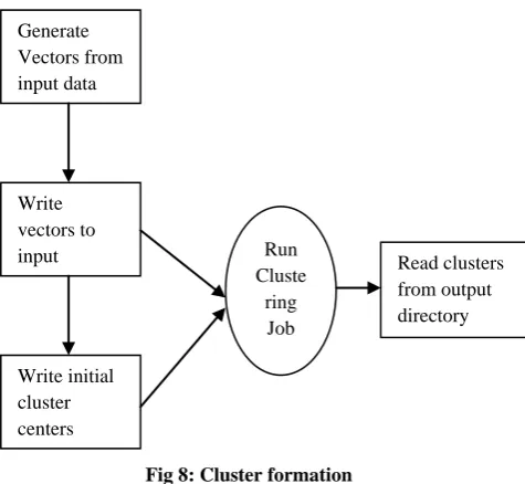
[image:7.595.311.564.94.390.2]It is the approach of unsupervised learning. Many times it may happen we don’t have any previous example, in that case we will try to form cluster on the basis of similarity or dissimilarity after the entrance of every new object. Sometime new object will belong to cluster and sometime they will make a new cluster.
Fig 8: Cluster formation
Given below figure show the different types of clustering approaches, these all are of different types and their approach is different from each other. Now I will display the names of algorithm which are used to form cluster, they are as follows: 1. K-means clustering
2. Centroid generation using canopy clustering 3. Fuzzy k-means clustering and Dirchlet clustering
[image:7.595.54.292.429.648.2]4. Topic modelling using latent Dirchlet allocation as a variant of clustering.
Fig 9: Clustering Approach
5.
CONCLUSION
Main idea behind writing this paper is to shows the various stages of big data analytics, what type of methods or algorithms we use at different stages during the whole process. Also discussed about the classification and clustering approaches.
6.
REFERENCES
[1] P. Rheingans and M. DesJardins, “Visualizing high-dimensional predictive model quality,” in Proceedings Visualization 2000. VIS 2000 (Cat. No.00CH37145), 2000, p. 493–496,.
[2] C.-W. Tsai, C.-F. Lai, H.-C. Chao, and A. V. Vasilakos, “Big data analytics: a survey,” J. Big Data, vol. 2, no. 1, p. 21, 2015.
[3] N. Tang, “Big data cleaning,” in Lecture Notes in Computer Science (including subseries Lecture Notes in Artificial Intelligence and Lecture Notes in Bioinformatics), 2014, vol. 8709 LNCS, pp. 13–24. [4] C. J. Zhang, L. Chen, Y. Tong, and Z. Liu, “Cleaning
uncertain data with a noisy crowd,” in Proceedings - International Conference on Data Engineering, 2015, vol. 2015–May, pp. 6–17.
[5] D. Peralta, S. Del Río, S. Ramírez-Gallego, I. Triguero, J. M. Benitez, and F. Herrera, “Evolutionary Feature Selection for Big Data Classification: A MapReduce Approach,” Math. Probl. Eng., vol. 2015, 2015.
[6] A. K. Jain, M. N. Murty, and P. J. Flynn, “Data clustering: a review,” ACM Comput. Surv., vol. 31, no. 3, pp. 264–323, 1999.
[7] M. Verleysen, “Learning high-dimensional data,” Limitations Futur. Trends Neural Comput., pp. 141–162, 2003.
Clustering
Hiera rchica l
Partiti onal
Categ orical
Large DB
Agglo merativ e
Divisi ve
Samp ling
Compr ession
Generate Vectors from input data
Write vectors to input directory
Write initial cluster centers
Run Cluste
ring Job
[8] P. Rheingans and M. DesJardins, “Visualizing high-dimensional predictive model quality,” in Proceedings Visualization 2000. VIS 2000 (Cat. No.00CH37145), 2000, p. 493–496,.
[9] C.-W. Tsai, C.-F. Lai, H.-C. Chao, and A. V. Vasilakos, “Big data analytics: a survey,” J. Big Data, vol. 2, no. 1, p. 21, 2015.
[10] N. Tang, “Big data cleaning,” in Lecture Notes in Computer Science (including subseries Lecture Notes in Artificial Intelligence and Lecture Notes in Bioinformatics), 2014, vol. 8709 LNCS, pp. 13–24. [11] C. J. Zhang, L. Chen, Y. Tong, and Z. Liu, “Cleaning
uncertain data with a noisy crowd,” in Proceedings - International Conference on Data Engineering, 2015, vol.
![Fig 1: Different stages of data preprocessing [3]](https://thumb-us.123doks.com/thumbv2/123dok_us/9299739.428462/2.595.64.271.69.294/fig-different-stages-data-preprocessing.webp)
![Fig 2: Representation of two dimensional features [4]](https://thumb-us.123doks.com/thumbv2/123dok_us/9299739.428462/3.595.317.540.629.725/fig-representation-dimensional-features.webp)