Forecasting the Grant Duration of a Patent using Predictive Analytics

Forecasting the Grant Duration of a Patent using

Predictive Analytics

Raman Dutt

Shiv Nadar University (Dept. of Computer Science) Shiv Nadar University

Uttar Pradesh, India

Vinita Krishna, PhD

Shiv Nadar University (School of Management) Shiv Nadar University

Uttar Pradesh, India

ABSTRACT

In the race for survival in an age of technological advancement and overspilling data, organizations are clamoring to use the eas-ily available data for better decision making. The arrival of the next generation of innovative and disruptive technologies has also led to patenting race. Companies are reorienting their business goals and strategies to maintain their competitive edge in the market. Patent data has been an obvious choice for analysis, leading to strategic technology intelligence. The advancement of Machine Learning and access to large amounts of patent data has led to a paradigm shift from traditional patent data analysis, methodologies and ap-proaches to novel procedures. This work aims to weigh the bene-fits & constraints of these approaches in patent analysis. In doing so, some of the important factors-the so called patent characteris-tics , cited in literature were identified as impacting the decision on grant duration of patent applications. A comprehensive compar-ative study of the prediction algorithms was also performed. Fi-nally, a quantitative study of the results is presented. This research is exploratory in nature and to the best of our knowledge, first of its kind in terms of research design and the context i.e analysis of dataset from a developing country (India) and the techniques used (ML/DL) in patent grant duration prediction.

General Terms

Data Science, Patent Analysis, Patent Forecasting

Keywords

business intelligence, data science, machine learning, predictive modelling, predictive model

1. INTRODUCTION

For a business organization, there are a plethora of reasons why it should file for patents for its products and services. In this highly competitive market, organizations are fighting to establish their hegemony in the market, make their product stand out and extract maximal profit from it. In order to achieve this, patenting their prod-ucts seems the most appropriate choice.

Some of the benefits that patents provide an organization are exclu-sive rights over products, higher return on investments, opportunity

to license or sell the invention, etc . Among these, the two most compelling reasons are strong market position and the first-mover advantage for the organization [29]. For instance, if two organiza-tions are planning to launch a similar product in the market, the organization successful in launching it first will draw the highest proportion of the user base while the companies following it would be left with the remaining market share.

Through these exclusive rights, companies are able to prevent oth-ers from commercially using their patented invention, thereby re-ducing the competition. The patent portfolio is a collection of all the applications filed for patents by an organization. This includes both the applications that have been granted as well as those that have been rejected for patents. Patent portfolios play an extremely important role in determining the technological strength of an or-ganization. Business partners, investors, and shareholders may per-ceive patent portfolios as a demonstration of the specialization and high level of expertise within a company [29].

Due to such immense importance of patents, it is necessary to in-vest in intelligent decision making. Patents are the most feasible approach for analyzing the breadth and depth of research and de-velopment within a company as the patent data provides insight to its competences [26]. The depth corresponds to the diversity of patents in an organization while the depth corresponds to the num-ber of patents in a particular domain. These two metrics are essen-tial for patent portfolio analysis.

2. RELATED WORK

2.1 Machine Learning and Natural Language Processing on the Patent Corpus

and introduced their patent data project under the National Bureau of Economic Research (NBER). This data is widely preferred and used because the assignees have been matched to unique identi-fiers of publicly listed firms, a characteristic that was missing from other academic datasets. This time-consuming element in the en-tire pipeline could be removed or at least alleviated with the help of automation. Recent advances in Machine Learning and Natural Language Processing could be used to automate this process of re-moving ambiguity. The major motivation behind this work was to provide a tool for automating certain steps in the process of disam-biguation and data manipulation. Apart from the above-mentioned tasks, the other areas of investigation that this work opens up are providing a measure of a novelty for the patents based on the first occurrence of a word in the patent corpus.

The first step was to collect the data from the USPTO. This was done by creating a python script that would scrape the data avail-able on the USPTO website. The scraped data is then cleaned and checked for consistency following which it is stored in a relational database. After storing the data and ensuring its consistency, the work on removing ambiguity was initiated.

Inventor disambiguation was treated as a clustering problem. In or-der to disambiguate names, a high intra-cluster similarity and low inter-cluster similarity was searched for among the patentinventor pairs. Both top-down and bottom-up approaches were applied to avoid incorrect lumping and splitting of inventors. Each patent was modeled as an unordered collection of that patents attributes. The occurrence of each attribute is used as a feature. A document-by-attribute incidence matrix was built which was extremely sparse be-cause a patent cannot possibly contain all the attributes from other patents in the dataset. In the incidence matrix, the presence of an attribute was indicated by a 1 whereas the absence was indicated by a 0. A submatrix was constructed from the incidence matrix for computing the correlation between the rows and columns. The lumping and splitting of inventor names across patents was determined by considering each inventor’s name, coinventors, geo-graphical location, overlap in CPC technology class, and assignee by the disambiguator. The results obtained using this approach are more or less accurate than the previous approaches to disambiguate the entire US patent corpus. The splitting rate obtained in this work was 1.9% as compared to 3.3% obtained by Li et al., 2014 [16] while at the same time, the lumping error rate obtained was 3.% as compared to 2.3%. This method is much simpler and runs much faster and has approximately 1/10th of the code of Lai et al.(2009) [12].

2.2 Technology Transfer using Predictive Patent Analysis

With the rise of international competition and the accelerated pace of technological advancements, companies try to maintain compet-itiveness in the market through effective innovation and are con-stantly on the lookout for new and emerging technologies. Compa-nies relied on the internal R&D for technological development but over time they havent been able to keep up with the momentum. It is becoming an increasingly difficult task for R&D practitioners to analyze emerging technologies due to the rapid pace of technolog-ical advancements. From a technology management point of view, identification of technological trends is very important for R&D re-searchers to manage their own technology and gain a competitive advantage in the market. It is the commercialization of that tech-nology which is their ultimate goal. To stay relevant in the market, companies are relying more and more on external sources for

tech-nological innovation mostly through open innovation technology transfers.

It is important to promote open innovation, since growing uncer-tainties in the world economy have seen a contraction of the tech-nology market [9] [14]. In the world of growing uncertainties in the global economy, it is becoming more and more important to promote open innovation to avoid the contraction of the technol-ogy market. Intellectual property has come to the centre of this phenomenon and patents are the key to open innovation. The rapid change in R&D environment has made the need for new methods of technology analysis very clear. Unlike the traditional R&D which is majorly focused on marketing strategies based on product devel-opment and sales, the new environment is marked with importance of marketing intangibles assets such as the intellectual property. The fundamental aspect of the commercialization of technology is the tech transfer phase. A great number of patents are filed and reg-istered every year out of which many enterprise-oriented patents are screened out through the registration process on grounds of creativ-ity, novelty and industrial applicability. Even though these rigorous selection processes are in place, the transfer of these patents is low compared to the total number of patents registered in a particular year. To deal with this, several methods were explored to build a predictive model for technology transfer using patent analysis. Choi et al. [3] trained a predictive model to reveal the quantitative relations between technology transfer and a range of variables in-cluded in the patent data. They achieve these results by conducting social network analysis, linear regression and decision tree mod-elling to create a model which is useful not only for prediction of technology transfers but also end up preventing mismatch errors from reviews of experts and prevent waste of R&D resources. Sev-eral other attempts have been made to ramp up R&D management and make it more efficient by employing predictive models based on statistical analysis and machine learning. Sohn and Moon [12] built a predictive structural equation model for that scores and gen-erates a technological commercial success index (TCSI). They also proposed a decision tree model, in their follow up, on the data en-velopment analysis (DEA) to evaluate the commercial success of a technology. Choi et al. [3] conducted a co-classification analysis of all patent data registered under the Korea Intellectual Property Office between 1988 and 2010. It was found that the number of patents kept on reducing as the convergence went on increasing, after analysing the convergence trends of technology.

Patent documents are categorized under text-heavy unstructured data which does not have a predefined data model. It is impor-tant to convert the data into a structured manner before any sort of analysis is performed on the dataset. This can be done using text mining, and natural language processing. This data can be analysed using decision trees or Social Network Analysis (SNA). SNA is a graph based analysis method which has vertices and edges and also employs a visualisation method based on graph theory. Further, re-gression analysis can be applied to the graph based results of the SNA.

2.3 Patent Number Forecasting by Regression on Cloud Storage Technology

var-ious distributions of patents in respective fields, monitor the trend of technological changes in the market, and compare competition level by employing statistical charts and graphs. Patent maps show macroscopic view of patents, and offer a company to determine the direction of R&D.

In the work by K Liu, Y Chen [18], a linear regression model was employed to forecast the number of patents being filed based on the number of inventors registering for those patents. The data for this work was collected by running various search queries on the US patent publication database. Different forms of queries were used to retrieve different data of different forms. Each query returned a dif-ferent number of results (hits) which were then used as the dataset for the work. This data was then analysed and organizations with greatest and least contributions in the number of patent applications were identified. The linear regression model was run on the three major contributors in the number of patent applications, namely, Microsoft, IBM and Yahoo. The results also show that the top two patentees, namely, Microsoft and IBM, are difficult to surpass in the coming years. This prediction is also in harmony with the present state Microsoft and IBM are well above any other organization in terms of number of patent applications.

This work demonstrated that a simple statistical method such as lin-ear regression can end up being a powerful method in this case and help in estimating how many patent applications should be filed by a company in a particular time period to achieve maximum success with their patent applications, which can further help in determin-ing the R&D budget and can help minimize losses in opportunity costs.

In linear regression, coefficient of determination determines how well data points fit a statistical model. The value of lies between 0 and the higher value of R square, the stronger explanation of the linear model and higher reliability. In case of Microsoft, the coeffi-cient of determination was 0.934, which shows high reliability. In case of IBM and Yahoo, the values were 0.913 and 0.9451 respec-tively.

3. PROBLEM DEFINITION

Patent grant duration is the amount of time it takes for an applica-tion to be successfully granted a patent. It is calculated as the time duration between date of filing of the application and the date of grant of the patent for that respective application. The study of the patent grant duration is important to follow the trends of a particu-lar technology by companies that make products using that technol-ogy. Therefore, deriving the relationship between the patent grant duration and factors which affect it are of utmost importance for an Intellectual Property (IP) savvy organization. In this technology-oriented environment, it is very crucial for the companies to build and maintain a strong patent portfolio to hold the desired mar-ket position and positive image for the organization. However, this topic has not been extensively covered in literature. By leveraging the advancements in machine learning and statistical studies, this challenge can be handled in a much more efficient manner. The motivation behind this work was to provide a business tool for companies to get a fair estimate of the duration (in days) for a filed patent application to be granted. Various factors which affect the duration of the grant of a patent are identified and also ranked according to their relevance or importance. Delay in patent grants can mean that companies with innovative and unique products have to wait longer to enter a particular market. This can have a huge impact on the business as the company can miss out on the first mover advantage and even the competitive edge. This could also

result in financial losses as it would be difficult to meet the cost incurred during the research and development of the product. Upon knowing the estimated grant duration of the application and the factors it depends on, the organizations can tweak those factors so that the estimated duration now lies in the required range. This can help the companies to get their applications granted in possibly a shorter duration of time which can be of immense value when it comes to maintaining their market position and patent portfolio status.

4. RESEARCH METHODOLOGY

The entire research methodology was divided into the following stages

-(1) Data Collection (2) Data Preprocessing

(3) Implementing the algorithms and feeding the data (4) Evaluating the results

(5) Quantitative analysis of the findings

4.1 Data Collection

Samples of patent data was collected from the Indian Patent website using the Indian Patent Advanced Search System (INPASS). The search system allowed us to query patent data from the database by applying filters such as Application Date, Title, Abstract, Applicant Country, Date of Filing, Grant Data etc. INPASS provides us with a total of 16 such filters to apply while querying the data. After a care-ful analysis, 4 features emerged out to give significant contribution towards predicting the grant date duration. Features such as ’Patent Number’, ’Filing Office’, ’PCT Application Number’, ’PCT Publi-cation Number’ were excluded because these do not directly affect the grant duration of an application. The 4 features selected are -(1) Inventor Country

(2) Applicant Country (3) Field of Invention (4) Application Date

Another featured ’Number of Days’ (or Grant Duration) was not explicitly provided but was calculated by us by subtracting the grant date and date of filing of the application. A description of the features is given in Table 1.

The INPASS search system provided the option to search for both Granted and Published patent applications. Since the grant duration for the patent applications was being predicted, only those applica-tions were considered which were actually granted patents. A total sample of 1000 granted patents between the years 2001 -2018 was collected based on a mix of judgemental and convenience sampling technique because the aim was very specific and data was collected manually.

Table 1. Description of Features

Feature Name Feature Description

Inventor Country The country where the product was invented Applicant Country The country where the application was filed Field of Invention The field under which the application was filed Date of Filing The date on which the application was filed Grant Date Date of Acceptance of the Patent Application Number of Days Time taken for the application to be accepted

are top filers at the Indian Patent Office. By capturing the essential factors, we intended to study, analyze and forecast the patterns in the data.

4.2 Data Preprocessing

Upon examining the data, it was observed that the all the fea-tures (’Applicant Country’, ’Field of Invention’, ’Inventor Coun-try’) were categorical in nature. Any data attribute which is cate-gorical in nature represents discrete values which belong to a spe-cific finite set of categories or classes.These discrete values can be text or numeric in nature. In any nominal categorical data attribute, there is no concept of ordering among the values of that attribute. For instance, a class label Inventor Country would not mean any-thing if it comes before say Field of Invention. Similarly, Applicant Country is not numerically greater than Inventor Country. In order to process these features, pandas python package [19] was used. This library provides a function ’get dummies’ which converts cat-egorical data into binary vectors which can be fed into the machine learning algorithms.

4.3 Implementing the algorithms and feeding the data

All the statistical algorithms were implemented using the Scikit-Learn library [21] (a python library for machine learning). The li-brary provides a collection of machine learning algorithms for dif-ferent tasks such as supervised and unsupervised learning. A re-sampling technique called K-Fold Cross Validation was also used which is used to evaluate machine learning models on a limited data sample. The value of k was chosen to be 10. The scikit-learn library also provides different metrics which have been used in this work to evaluate the performance of different models. Following algorithms were used for analysis.

(1) Support Vector Machines

A Support Vector Machine (SVM) [27] is a discriminative clas-sifier formally defined by a separating hyperplane (Fig. 1.). In other words, given labeled training data (supervised learning), the algorithm outputs an optimal hyperplane which categorizes new examples. In this algorithm, each data item is plotted in an n-dimensional (where n is number of features) with the value of each feature being the value of a particular coordi-nate. The support vector machine can also be used as a regres-sion method. In the case of regresregres-sion, a margin of tolerance (epsilon) is set in approximation to the SVM.

(2) Decision Tree Regression

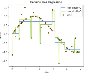
In decision trees [22], the goal is to create a model that predicts the value of a target variable based on several input variables. Each interior node corresponds to one of the input variables; there are edges to children for each of the possible values of that input variable. Each leaf represents a value of the target variable given the values of the input variables represented by the path from the root to the leaf (Fig. 2). A decision tree

Fig. 1. Support Vector Regression [27]

is built top-down from a root node and involves partitioning the data into subsets that contain instances with similar values (homogeneous). Standard deviation was used to calculate the homogeneity of a numerical sample.

Fig. 2. Decision Tree Regression [15]

(3) Gradient Boosting Regression

Gradient boosting [7] is a machine learning technique for re-gression and classification problems, which produces a predic-tion model in the form of an ensemble of weak predicpredic-tion mod-els, typically decision trees (Fig. 3).

(4) Random Forest Regression

Fig. 3. Gradient Boosting Regression [8]

Fig. 4. Random Forest Regression [25]

(5) AdaBoost Regression

An AdaBoost regressor [6] is a meta-estimator that begins by fitting a regressor on the original dataset and then fits addi-tional copies of the regressor on the same dataset but where the weights of instances are adjusted according to the error of the current prediction (Fig 5.). As such, subsequent regressors focus more on difficult cases. This algorithm is sensitive to out-liers and is thus useful to check for outout-liers in the dataset.

Fig. 5. AdaBoost Regression [4]

(6) Bagging Regressor

Bootstrap aggregating [2], also called bagging, is a machine learning ensemble meta-algorithm designed to improve the stability and accuracy of machine learning algorithms used in statistical classification and regression. It also re-duces variance and helps to avoid overfitting. It is a special case of the model averaging approach. Since the dataset in this work is not very large, bagging plays an important role so as to ensure that the model is not overfitting on the data.

(7) Ridge Regression

In simple linear regression, the individual variable importance is not considered. Ridge Regression [11] is a technique for analyzing multiple regression data that suffer from multi-collinearity. When multicollinearity occurs, least squares estimates are unbiased, but their variances are large so they may be far from the true value. By adding a degree of bias to the regression estimates, ridge regression reduces the standard errors. It is hoped that the net effect will be to give estimates that are more reliable. This method helps us study the importance of different features which is of immense importance with respect to this work.

(8) Lasso Regression

Lasso regression [28] is a type of linear regression that uses shrinkage. Shrinkage is where data values are shrunk towards a central point, like the mean. The lasso procedure encour-ages simple, sparse models (i.e. models with fewer parame-ters). This particular type of regression is well-suited for mod-els showing high levmod-els of muticollinearity or when you want to automate certain parts of model selection, like variable se-lection/parameter elimination.

(9) Multi Layer Perceptron

A multilayer perceptron (MLP) is a class of feedforward arti-ficial neural network. A MLP consists of at least three layers of nodes: an input layer, a hidden layer and an output layer. Except for the input nodes, each node is a neuron that uses a nonlinear activation function. MLP utilizes a supervised learn-ing technique called backpropagation [23] for trainlearn-ing (Fig 6.). It can distinguish data that is not linearly separable. The MLP used in this work consisted of two hidden layers and a learning rate of 0.1.

(10) Auto-sklearn

Automated machine learning (AutoML) is the process of au-tomating the end-to-end process of applying machine learning to real-world problems. A typical workflow of a machine learn-ing application involves data pre-processlearn-ing, feature engineer-ing, feature extraction, and feature selection. The developer also also needs to perform model selection for testing which model performs better and also hyperparameter optimization to further improve the results and maximize the predictive per-formance of the models. AutoML was proposed as an artificial intelligence-based solution, automating the end-to-end process of applying machine learning and offers the advantages of pro-ducing simpler solutions, faster creation of those solutions, and models that often outperform models that were designed by hand.

Auto-sklearn [5] is an open-sourced, python tool that is built on the principles of auto-ml. It is built around the scikit learn li-brary [21]. Auto-sklearn contains around 110 hyperparameters and tuning them for optimization can be a very time consum-ing process. In order to jumpstart this process, meta-learnconsum-ing is employed to start from good hyperparameter settings for pre-vious similar datasets. Another point of advantage that auto-sklearn offers is that it automatically construct ensembles, in-stead of returning a single model. This results in the creation of small, powerful ensembles with increased predictive power and robustness.

4.4 Evaluating the Results

The metrics used for the evaluating different machine learning models were Mean Absolute Error (MEA), Root Mean Squared Error (RMSE) and R2 _{score. All the error values calculated here}

are in number of days.

Mean absolute error is the average of absolute values differences between the true values and the values predicted by the machine learning model on the test set. The mean absolute error is robust to outliers. MEA is not much affected by any data point that is very far from the majority of the data points.

Root Mean Squared Error (RMSE) is the square root of average of square of differences between the true values and the values pre-dicted by the machine learning model on the test set. This error is smoothly differentiable and makes it easier to perform mathemati-cal operations. The RMSE is sensitive to outliers and penalizes the higher difference between the true and predicted values much more than MAE.

R Squared and Adjusted R Squared explain how well your selected independent variable(s) explain the variability in your dependent variable(s). The smaller the value of R Squared, the poorer is the model. Adjusted R also shows how well terms fit a curve or line but adjusts for the number of terms in a model.

The results in Table 2. show that the ensemble created using au-tomated machine learning (Auto-Sklearn) gave the best results and outperformed even the deep learning algorithm (multi layer percep-tron). The specifics of the ensemble are shown in Table 3. The first pipeline used Extra Trees as a pre processor choice and K Nearest Neighbours (KNN) as the regressor. This pipeline was given a weight of 0.54 in the final ensemble. The second pipeline used a different pre processor which was feature agglomeration and the same regressor. This pipeline was given a weight of 0.32 in the final ensemble. The third pipeline was constructed using fast ICA as the pre processor and Libsvm-SVR as the regressor and was given a weight of 0.14 in the final ensemble.

Table 2. Evaluation Metrics on the Test Data

Algorithm RMSE MAE R2_Score

Support Vector Regression 1061.42 902.17 -0.073 Decision Tree Regression 1912.36 735.52 -2.48 Gradient Boosting Regression 1912.36 735.52 -2.48 Random Forest Regression 2009.19 740.65 -2.84 Adaboost Regression 2878.54 1307.64 -6.89 Bagging Regression 1801.04 732.13 -2.09 Ridge Regression 1007.26 769.00 0.033 Lasso Regression 1023.13 770.01 0.002 Multi Layer Perceptron 834.23 680.18 -0.62 Auto-Scikit Learn 778.30 590.30 0.42

Table 3. Auto-Sklearn Ensemble

Pipeline Weight Pre-Processor Choice Regressor

Pipeline 1 0.54 Extra Trees KNN Pipeline 2 0.32 Feature Agglomeration KNN Pipeline 3 0.14 Fast ICA Libsvm SVR

5. DISCUSSION

Several predictive models were developed for the task of forecast-ing the patent grant duration. These models have also been eval-uated and compared so as to come up with the algorithm which gives the best results (least error values). The algorithm which gives the best results is developed using the principles of automated ma-chine learning, which is an artificial-intelligence based solution for automating the different steps involved in developing a machine learning application. Apart from this, this work is not just limited to machine learning algorithms but have deep learning techniques have also been used which learn by creating a more abstract repre-sentation of data.

From the results, we see that the ensemble created by auto-sklearn gave the least value for the root mean squared error (RMSE) and the mean absolute error (MAE). The best R2 _{score was also given by}

the same ensemble. Other models such as Random Forest, Gradient Boosting and Adaboost failed to perform well on the dataset. Multi Layer Perceptrons (MLP) gave the second best performance after the auto-sklearn ensemble. Ridge Regression and Lasso Regression gave almost similar results and came after the MLP in terms of performance. Support Vector Machines performed better than the ensemble methods but not better than Lasso and Ridge Regression. The deep learning method (Multi Layer Perceptron) performed bet-ter than most of the algorithms but not with a significant margin while the ensemble created using auto-sklearn outperformed every other algorithm. The small size of the dataset and the small num-ber of features considered is a possible explanation for this because neural networks usually require much larger amount of data [24] than what is considered for this work. On the other hand, auto-sklearn is a result of some of the most recent advancements in the field of machine learning, automatically selects the best models with most optimum hyper-parameters for the final ensemble.

6. REFERENCES

[1] David M Blei, Andrew Y Ng, and Michael I Jordan. Latent dirichlet allocation.Journal of machine Learning research, 3(Jan):993–1022, 2003.

[3] Jae Young Choi, Seongkyoon Jeong, and Kyunam Kim. A study on diffusion pattern of technology convergence: Patent analysis for korea. 2015.

[4] Akash Desarda. Understanding adaboost.

[5] Matthias Feurer, Aaron Klein, Katharina Eggensperger, Jost Springenberg, Manuel Blum, and Frank Hutter. Efficient and robust automated machine learning. InAdvances in neural in-formation processing systems, pages 2962–2970, 2015. [6] Yoav Freund, Robert E Schapire, et al. Experiments with a

new boosting algorithm. Inicml, volume 96, pages 148–156. Citeseer, 1996.

[7] Jerome H Friedman. Greedy function approximation: a gradi-ent boosting machine.Annals of statistics, pages 1189–1232, 2001.

[8] Prince Grover. Gradient boosting regression.

[9] Stefan Hack and Christian Berg. The potential of it for corpo-rate sustainability.Sustainability, 6(7):4163–4180, 2014. [10] Bronwyn H Hall, Adam Jaffe, and Manuel Trajtenberg.

Mar-ket value and patent citations.RAND Journal of economics, pages 16–38, 2005.

[11] Arthur E Hoerl and Robert W Kennard. Ridge regression: Bi-ased estimation for nonorthogonal problems.Technometrics, 12(1):55–67, 1970.

[12] Fang-Ming Hsu and Chao-Chih Hsueh. Measuring relative ef-ficiency of government-sponsored r&d projects: A three-stage approach.Evaluation and program planning, 32(2):178–186, 2009.

[13] Nitin Kumar Kain. Understanding of multilayer perceptron (mlp).

[14] Hideki Kobayashi, Masahiro Kato, Yukishige Maezawa, and Kenji Sano. An rd management framework for eco-technology. 2011.

[15] Scikit Learn. Decision tree regression.

[16] Guan-Cheng Li, Ronald Lai, Alexander DAmour, David M Doolin, Ye Sun, Vetle I Torvik, Z Yu Amy, and Lee Fleming. Disambiguation and co-authorship networks of the us patent inventor database (1975–2010).Research Policy, 43(6):941– 955, 2014.

[17] Andy Liaw, Matthew Wiener, et al. Classification and regres-sion by randomforest.R news, 2(3):18–22, 2002.

[18] Kuotsan Liu and Yingching Chen. A study of patent numbers forecasting by linear regression on cloud storage technology. [19] Wes McKinney.Python for data analysis: Data wrangling with Pandas, NumPy, and IPython. ” O’Reilly Media, Inc.”, 2012.

[20] Subba Moorthy and Douglas E Polley. Technological knowl-edge breadth and depth: performance impacts. Journal of Knowledge Management, 14(3):359–377, 2010.

[21] Fabian Pedregosa, Ga¨el Varoquaux, Alexandre Gramfort, Vincent Michel, Bertrand Thirion, Olivier Grisel, Mathieu Blondel, Peter Prettenhofer, Ron Weiss, Vincent Dubourg, et al. Scikit-learn: Machine learning in python.Journal of ma-chine learning research, 12(Oct):2825–2830, 2011.

[22] J. Ross Quinlan. Induction of decision trees.Machine learn-ing, 1(1):81–106, 1986.

[23] David E Rumelhart, Geoffrey E Hinton, and Ronald J Williams. Learning internal representations by error propa-gation. Technical report, California Univ San Diego La Jolla Inst for Cognitive Science, 1985.

[24] Ida Jessie Sagina. Why go large with data for deep learning? [25] Tavish Srivastava. Tuning the parameters of your random

for-est model.

[26] Arho Suominen, Hannes Toivanen, and Marko Sepp¨anen. Firms’ knowledge profiles: Mapping patent data with un-supervised learning. Technological Forecasting and Social Change, 115:131–142, 2017.

[27] Johan AK Suykens and Joos Vandewalle. Least squares sup-port vector machine classifiers. Neural processing letters, 9(3):293–300, 1999.

[28] Robert Tibshirani. Regression shrinkage and selection via the lasso.Journal of the Royal Statistical Society: Series B (Methodological), 58(1):267–288, 1996.

[29] World Intellectual Property Organization WIPO. Reasons for patenting your inventions.