Interior-Point Methods Applied to the Predispatch
Problem of a Hydroelectric System with
Scheduled Line Manipulations
Silvia M. S. Carvalho, Aurelio R. L. Oliveira University of Campinas, Campinas, Brazil
Email: [email protected], [email protected]
Received March 12, 2012; revised April 13, 2012; accepted April 27, 2012
ABSTRACT
Transmission line manipulations in a power system are necessary for the execution of preventative or corrective main- tenance in a network, thus ensuring the stability of the system. In this study, primal-dual interior-point methods are used to minimize costs and losses in the generation and transmission of the predispatch active power flow in a hydroelectric system with previously scheduled line manipulations for preventative maintenance, over a period of twenty-four hours. The matrix structure of this problem and the modification that it imposes on the system is also broached in this study. From the computational standpoint, the effort required to solve a problem with or without line manipulations is similar, and the reasons for this are also discussed in this study. Computational results sustain our findings.
Keywords: Interior-Point Methods; Scheduled Line Manipulations; Hydroelectric Systems; The Brazilian Power System
1. Introduction
In a power system, continual improvements in opera- tional conditions are always sought; however, to achieve such improvements, constant maintenance and improve- ment work in the network is required, and scheduled shut-downs are sometimes required. Maintenance is ne- cessary to avoid electrical short circuits and overloads. Thus, the objective is to ensure the continual supply of electric power, with the fewest interruptions of the short- est duration possible, thus maintaining the service levels required by the legislation.
For instance, in Brazil the System Operation Center (COS) is responsible for executing, authorizing and su- pervising scheduled and emergency line manipulations in the power transmission system, as well as for monitoring the system and reestablishing the power grid in the event of isolated or generalized contingencies. These activities, executed in real time, require situational awareness and management of the execution of the necessary line mani- pulations, with the aim of ensuring the integrity of per- sonnel and installations, whilst guaranteeing the reliabi- lity of the system and the continuity and quality of sup- ply.
In this study, the predispatch will be modeled on a twenty-four hour period, representing the dispatch of a single day, and line manipulations will be an input data
point; in other words, they will already have been sche- duled, and thus the line manipulations considered herein will be of a preventative nature. It is important to empha- size that there are other types of manipulations, such as generator shut downs, tap changing procedures and fle- xible alternating current transmission system (FACTS) adjustments, but these are not considered in this study.
Furthermore, by making use of the speed and robust- ness of interior-point methods [1-3], the intention is to obtain more efficient implementations for predispatch by means of exploiting the matrix structure of the resulting system.
2. The Predispatch Problem
Predispatch is a short-term operational problem, in this case, short-term refers to one-week, or even one-day, planning. The intention is to fulfill demands and satisfy the energy targets that have been defined in long-term planning.
A predispatch system with m buses, n lines and g ge- nerators, where line manipulations are considered, can be modeled in the following manner:
1 1
min max min max
1 min 2 2 , 0 , , 1, , t t
t k k t k k t k
k k
k k
k k k k k
k k
k k
t k k
R f Q p c p
f p
A f E p d
X f
f f f p p p
p q k t
(1) where, n1
f represents the active power flow;
g 1
p represents the active power generation;
g g
Q represents the quadratic component of the generation cost;
cg1
represents the linear component of the ge- neration cost;
Rn n
represents the diagonal matrix of line re- sistance;
dm1
represents the active load;
n m 1n
represents the reactance active matrix;
X
E represents a matrix of order m × g, with each column containing exactly one element equal to 1 and all other elements equal to 0;
Am n
represents the incidence matrix of the transmission network;
g
represents the flow and active power generation limits, respectively;
max, min n 1, max, min 1
f f p p
and objective function weight constants;
g 1
q represents the power generation target est- ablished in long-term planning.
For this model, the two objective function components are quadratic with separable variables. The first com- ponent represents the value of the transmission losses. The second component characterizes the generation cost of the plants [5].
Problem (1) may be simplified using changes in vari- ables [6] and adding slack variables, thus we get the pri- mal problem in its standard form:
1 1 max max 1 min 2 2 , , ,, 0, , 0
1, ,
t t
t k k k t k k t k
k
k k
k k k k k
k k k
k k k k
p f
t
k k
k k k
p f
k
R f p Q p c p
f
A f E p d
X f l
f s f p s p
f s
p q p s
k t
Whose respective dual problem may be expressed as:
max max 1 1max ˆ ( )
( )
2 2
ˆ
, , , 0
, free 1, ,
t
t t
t k k k
k t
p a
f f
k
t
t k k t k
k
k
t k k k k
f f f f
t k k k k
p a p p
f k k k k
p p f f k
a f
y f w p w q
d
p Qp Rf
f
B y w Rf z c
E y w y Qp z c
z w z w
y y k t
y (2)Matrix B, formed by the juxtaposed rows of the in- cidence and reactance matrices, is no longer constant throughout the time intervals t, and may be partioned as:
A B X
In a more detailed form:
T N B XT XN where
A T N and
X XT XN
With this partitioning, the columns of incidence matrix
A are divided so that T contains the edges of a spanning tree and N is formed by the remaining edges, which be- long to the co-tree [7], and the reactance matrix X is par- titioned in a similar manner.
Matrices B and E vary in accordance with the time in-tervals (Bk and Ek), reflecting the modifications to the networks and buses by line manipulations carried out throughout the study window. The reason that these ma- trices vary according to the time intervals is that the net- work is no longer constant throughout these t-intervals. Every time a line manipulation occurs, matrix B formed by the juxtaposed rows of the incidence and reactance matrix, and matrix E of order m × g should vary in accor- dance with the changes imposed on the network.
The primal-dual interior-point methods consist of the application of Newton’s method to the optimality con- ditions [8]; therefore, the following linear system is ob- tained: ~ 1 1 ˆ , ˆ , , .
k k k k
f f
k k
p p
t k k k
y
f f f
k k k k
p a p g
f
k k k k k k k k
wf p zp
f f f f
p t
k k k k k
p p p wp m
k
Bdf Edp r df ds r
dp ds r
B dy dw Rdf dz r
Edy dw dy Qdp dz r
S dw W ds r P dz Z dp r
S dw W ds r dp r
when several variable substitutions are made, we get:
(4)
whose direct solution requires great computational effort,
because,
1 1
1 1
1
1 1
ˆ ( )
ˆ
t
t k
k k
a p
p p
k t
k t
p b
k
dy E D
D D
rm D r E M r
1k t k
f D
M B B D has the dimension of the number of generators.
3. Scheduled Line Manipulations
Line manipulations are executed with the intention of adapting the transmission network to the load variation
anipulation azilian power system
our to six line manipulations are executed per day. The changes considered herein are other words,
Matrix B is formed by the juxtaposed rows of the in- onstant
thro e that a line
the number of rows and dya has the dimension of
(variation of the power demand) throughout the day. In most time intervals, line m s are not executed
in the Br , which means that the
transmission network rarely alters from one time interval to another, normally f
called preventative line manipulations; in
alterations to the network so that maintenance can be carried out and power blackouts avoided.
3.1. Study of the Matrix Structure for the Problem with Line Manipulations
We assume that in this system, i previously scheduled line manipulations take place over t time intervals, where each time interval corresponds to the period of one hour, and i line manipulations are few with the average value ranging from zero to six, which is typical of the Brazilian system.
cidence and reactance matrices, and is no longer c ughout t time intervals, because every tim
manipulation is executed, we can infer that a row and a column of matrix B are removed (inserted), in the event that more than one line manipulation occurs in the same time interval, more rows and columns of matrix B are re- moved (inserted). Thus, when we consider a system with line manipulations at different time intervals, we will use the following representation:
k k
k A B
B
where,
1, 2, , 24
k
Every time a line manipulation occurs during interval
k, matrix B will have its size modified, because it is formed by the incidence matrix, which represents the net- work topology, and by the reactance matrix. Therefore, if
a line is disconnected from the grid at time k, then the incidence matrix should represent the network at that exact instant in time; in other words, a column of A is ed, therefore the reactance associated with that row should also be extracted from the matrix.
eliminat
As the size of matrix B may be modified with each line manipulation, we must adjust the system to these changes; in other words, in order to obtain the product and the sum total with B, the size of some of the matrices involved in the system should also be altered.
The initial objective is to solve the linear system (4), but for this we realize that too much computational effort would be necessary to solve it directly, because in the first equation, we have the following matrix:
1
k k k k t k
f
M B D B D
whose size is the number of rows at instant t, while the size of vector dya is the number of generators. A more efficient solution follows these steps [6]:
Step 1) Consider a matrix Bk, consisting of matrix Bk
and canonical vector ej, thus
k k
j
B B e
(note that this matrix is square and nonsingu r). Step 2) A row and a column is added to matrix
la
1 k fD ,
in order to adjust its size for multiplication of the ma- trices.
Step 3) In matrix Dk, remove the jth row and the jth
co
ingly, we are removing a generation bus from the matrix and its size is not altered, rather only replaced with zero in the oved jth row and lumn, with j varying from 1, 2, ···, m, where its inter- sections cannot be zero. Accord
rem column.
Thus
Dkf 1
Dkf of Dk Dk and of, a ma becomes ktrix M
M and rewritten as
1( )
k k k t k
f D
M B B D
which has the size (n + 1)×(n + 1), and the vector
11
k k k
a p b
f D
r r B r E D r Step 4) We define:
f ( )1 k k
k k t k
f
dy r
D
B B D
(5)
this system will be solved in two stages [9 We will first solve the following linear system:
]:
tk D k k
B B dy r
f f
Accordingly, the “inversions” of and
m is important to emphasize that we
are supposing that in t time intervals, i-scheduled line k
B
k tB
manipulations take place; in other words, the m and vary throughout the interval
.
atrices , as a k
B
k tB
function of this number of line manipulations In order to solve (5), we have dy which is
difficulties, using, for example, the LU factor of difficulties, using, for example, the LU factor of found without
h does vary throughout the iterations. In alger- braic form
found without
h does vary throughout the iterations. In alger- braic form
whic
whic not
, we write: not , we write:
1. t
k k
f D
dy B B r
The Sherman-Morrison-Woodbury formula [10] is used to solve the linear system (5), in this case the computation of invertible matrix Mk
1
t
1 1
1 1
1 t 1C C U V C
C USV S V C U
where U and V are matrices of size p × q and S is of size
q × q, and therefore suitable for our problem C
t
t k k kf
B D B
and
t k
USV D
S is a diagonal matrix of size g × g, whose elements are those that belong to matrix k
Matrix its columns removed from the identity matrix
k
B
D
U has
k k k f k k k
B
B
t t V U
Therefore,
k
1M is expressed as:
1
11
ˆ ˆ
f
t
t k t
k k k k k k
f E Z
B D B E
1 1 t k
t
B D D
B D
B D
f
where
11 ˆ
ˆk t k k k t k. f
Z S E B D E
B
at Z
e size of t n of Z
plication of t
lying
ready applied in t
Note th is a symmetric positive-definite matrix, th he number of generators. Therefore, the putatio is simple, because the matrix enables he Cholesky decomposition [11 d has a relatively small size.
Multip the Sherman-Morrison-Woodbury equa- his context, by we get:
with com
the ap ] an
tion, al
1
1
1 ˆ 1
.
t t
k k k k k ˆ k
f f
dy dy B f B E Z E dy
Observe that the matrices Mk L Uk k can be decom- posed once only before the iterative process, in an iden- tical fashion to what can be done with matrix B, in the case of the problem without line manipulations.
3.2. Implementation Details for the Developed Methods
In order to devinterior-points methods for a system with
line manipulations, the network s to be adap d. With each line manipulation carried out, a row an a
co ved) from m
d), r
It is worth em sizing that as the spanning tree is not
t. te d need
lumn can be inserted (remo atrix B. The spanning tree is represented by matrix T and must not be modified; in other words, only the branches be- longing to matrix N, formed by the additional branches of the spanning tree, can be connected (disconnecte thus facilitating implementation and resulting in greate computational efficiency.
pha
unique and the line manipulations are previously known, any branch may be manipulated, and all this would re- quire is the construction of another spanning tree, as long as the branch to be manipulated did not belong to i
The tests undertaken in this study use the starting point shown in the Equation (6). This was defined as in [12], which presented satisfactory results in previous experi- ments.
max 0 f
f
max 0
0 0 0 0
1 2 3 4
0 0
2
2
0
p p
y y y y
1 1 0 0 2 2 0 0
( )
.
z w R I e
z w e
z w e
(6)
3 3
4. Computational Results
The networks in which the tests were carried out in- clude the IEEE30 bus system, representing the Midwest of the United States of America, and also
South-Southeastern-Central-West region wi
(SSECO1732) and the Brazilian interconnected system, consisting of 1993 buses.
In the computation experiments carried out, the pri- mal-dual interior-point method was used and tests were n with the number of line manipulations varying from which is what normally
stem.
ipulated in the grids were cho- se
ere to di
the Brazilian th 1732 buses
ru
zero to six over a 24-hour period,
happens in practice in the Brazilian power sy
The implementation was developed using Matlab 7.0, with a precision of 10–3, in order to satisfy the optimal conditions of the problem. The computer has an Intel Centrino Core 2 Duo processor, with 4 GB of RAM and a speed of 2.13 GHz.
The branches to be man
n randomly, and we emphasize that several tests were carried out and drastic differences from one test to an- other were noted, because the number of iterations and the computational time can vary significantly, depending on the branch that is being manipulated. If we w
would have to find a new way of fulfilling the demand, thus reflecting on the number of iterations. However, other reasons may be responsible for the increase in the computational effort, because depending on the branches m
branch with a high flo
anipulated, the network resulting from these manipula- tions may not adapt very efficiently.
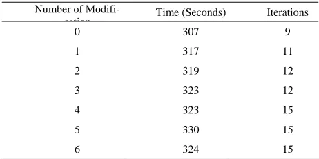
The first column of the Tables 1, 2 and 3 pertains to the number of manipulations and they are accumulative; for example, in the event of three manipulations, it con- sists of the branches previously manipulated (1 and 2) plus the new third branch.
Note that in all the tests carried out, the line manipu- lations represent a greater computational effort, but one that is acceptable due to the amount of support they pro- vide to the grid. The number of iterations necessary for convergence may vary significantly, depending on the branch that is being manipulated. If a
[image:5.595.56.288.330.445.2]w is disconnected, the grid will have to find a new
Table 1. IEEE30 system.
Number of
Modifi-cation Time (Seconds) Iterations
0 0.32 3
1 0.42 4
2 0.42 4
3 0.40 4
4 0.49 5
5 0.48 5
6 0.48 5
Num
odifi-Table 2. SSECO1732 system.
ber of M
cation Time (Seconds) Iterations
0 243 9
1 246 10
2 250 10
3 255 12
4 259 12
5 254 13
6 255 12
. B em.
Num
odifi-Table 3 razil 1993 syst
ber of M
cation Time (Seconds) Iterations
0 307 9
1 317 1
2 319 2
3 323 2
4 323 5
5 330 5
6 324 15
way through th nd, reflecting
on quently he
c ow actors re-
sponsible for this increase, because depending on the branch that is being manipu resulting net- work, grid aptation may not efficient.
In Tabl , the fourth manipulation was carried out in the branch ith the greatest f n the grid; no hat in this case, t number of iterations and the computational time are greater compared evious mani tions, therefore nipulating branc ith this characteristic
ifications in the net- ing from zero to six over a 24-hour , it is supposed that all changes in the
urrence of a line manipulation, a column in th
the modifications in the pr
this depends heavily on the br
for the method. The efficiency of the methodology used
1 1 1 1 1
e network to fulfill the dema the number of iteratio
omputational time. H
ns and, conse ever, other f
, on t may be
lated and its
ad be very
e 1
w he
low i te t
to pr pula
ma hes w
becomes a problem that is more challenging to solve. Similar event occurred in Table 3.
5. Conclusions
In this study, interior-point methods are used to solve a predispatch problem in a hydroelectric system. This re- search contributes to solving this problem with transmis- sion line manipulations. When these manipulations take place, the topology of the network is altered. The char- acteristics of this problem and its importance to the Bra- zilian power system have been the drivers behind this research.
In practice, the number of mod work is small, vary
period. In this study
network are known in advance. Thus, the matrices asso- ciated with the problem can be analyzed and decomposed before the interior-point methods are applied. An identi- cal approach has been taken by other authors for a sce- nario without manipulations.
Line manipulations represent the disconnection and/or return to operational status, of certain transmission lines. For each occ
e incidence matrix and a row in the reactance matrix are removed. The methodology used in the development of this study is the primal-dual interior-point method, because this presents satisfactory results for optimum power flow problems.
From the computational standpoint, the effort to solve a problem with or without modification in network to- pology is similar. Even with
oblem matrix, the number of linear systems that need to be solved is still the same, compared to the problem without manipulations. Furthermore, the number of itera- tions necessary for the convergence of the interior-point method depends on how important the manipulated bran- ches are to the grid.
The new method does not result in greater costs, al- though it is known that
[image:5.595.56.287.618.733.2]isting approaches that consider sche- du
nowledgements
. Innorta and R. Ricci, “The Flexibility of wer Flow Algorithms Facing s,” Electrical Power E Energy
in this study may be proven not only by means of con- vergence, but also for non-convergence of some of the tests carried out. Accordingly, it is possible to prove that the implementation actually optimizes the problems co- vered.
There are other ex
led transmission lines manipulation. For instance, line manipulation can be simulated. In this case, there is not network topology modification as oppose of the adopted approach. However, it presents stability difficulties and higher computational cost.
Thus, the solved model gets much closer to the actual problem with an insignificant additional computational effort, and without presenting any issues regarding nu- merical stability.
6. Ack
The authors would like to acknowledge the support given to their researches and studies by the Brazilian National Research Council (CNPq), the Brazilian Ministry of Education agency for graduate studies (CAPES) and the Research Foundation of the State of São Paulo (FAP- ESP).
REFERENCES
[1] A. Garzillo, M
Interior Point Based Po Critical Network Situation
Systems, Vol. 21, 1999, pp. 579-584.
[2] J. A. Momoh, M. E. El-Hawary and R. Adapa, “A Re- view of Selected Optimal Power Flow Literature to 1993, Part II Newton, Linear Programming and Interior Point Methods,” IEEE Transactions on Power Systems, Vol. 14, No. 1, 1999, pp. 105-111. doi:10.1109/59.744495
[3] V. H. Quintana, G. L. Torres and J. M. Palomo, “Interior Point Methods and Their Applications to Power Systems: A Classification of Publications and Software Codes,”
IEEE Transactions on Power Systems, Vol. 15, No. 1, 2000, pp. 170-176. doi:10.1109/59.852117
[4] T. Ohishi, S. Soares and M. F. Carvalho, “Short Term Hydrothermal Scheduling Approach for Dominantly Hydro Systems,” IEEE Transactions on Power Systems, Vol. 6, No. 2, 1991, pp. 637-643. doi:10.1109/59.76707
[5] S. Soares and C. T. Salmazo, “Minimum Loss Predis- patch Model for Hydroelectric Systems,” IEEE Transac- tions on Power Systems, Vol. 12, No. 3, 1997, pp. 1220- 1228. doi:10.1109/59.630464
[6] A. R. L Oliveira, S. Soares and L. Nepomuceno, “Opti-mal Active Power Dispatch Combining Network Flow and Interior Point Approaches,” IEEE Transactions on Power Systems, Vol. 18, No. 4, 2003, pp. 1235-1240. doi:10.1109/TPWRS.2003.814851
[7] R. Ahuja, T. Magnanti and J. B. Orlin, “Network Flows,” Prentice Hall, Englewood Cliffs, 1993.
y- erturbing Parameter,”
1190
[8] S. J. Wright, “Primal-Dual Interior Point Methods,” SIAM Publications, Philadelphia, 1996.
[9] L. M. R. Carvalho and A. R. L. Oliveira, “Primal-Dual Interior Point Method Applied to the Short Term H droelectric Scheduling Including a P
IEEE Latin America Transactions, Vol. 7, No. 2, 2009, pp. 533-538. doi:10.1109/TLA.2009.536
ress, Oxford, 1986.
work Flow [10] I. S. Duff, A. M. Erisman and J. K. Reid, “Direct Methods
for Sparse Matrices,” Clarendon P
[11] G. H. Golub and C. F. Van Loan, “Matrix Computations,” 2nd Edition, The Johns Hopkins University Press, Balti- more, 1989.
[12] A. R. L. Oliveira, S. Soares and L. Nepomuceno, “Short Term Hydroelectric Scheduling Combining Net