Techno economic analysis of global power quality mitigation strategy for provision of differentiated quality of supply

Techno-economic analysis of global power quality

mitigation strategy for provision of differentiated quality of

supply

LIAO, Huilian <http://orcid.org/0000-0002-5114-7294> and JOVICA, Milanonic

Available from Sheffield Hallam University Research Archive (SHURA) at:

http://shura.shu.ac.uk/23225/

This document is the author deposited version. You are advised to consult the

publisher's version if you wish to cite from it.

Published version

LIAO, Huilian and JOVICA, Milanonic (2018). Techno-economic analysis of global

power quality mitigation strategy for provision of differentiated quality of supply.

International Journal of Electrical Power and Energy Systems, 107, 159-166.

Copyright and re-use policy

See

http://shura.shu.ac.uk/information.html

Sheffield Hallam University Research Archive

Techno-Economic Analysis of Global Power Quality Mitigation Strategy

for Provision of Differentiated Quality of Supply

Huilian Liao

, Jovica V. Milanović

a_{Power, Electrical and Control Engineering Group, Sheffield Hallam University, Sheffield, S1 1WB, UK}

bSchool of Electrical and Electronic Engineering, The University of Manchester, PO Box 88, Manchester, M60 1QD, UK

* corresponding author: [email protected]

Abstract

This paper presents a comprehensive methodology for techno-economic assessment of power quality (PQ) mitigation solutions, both network-based and device-based, and proposes an optimisation-based PQ mitigation strategy for delivering differentiated PQ in networks integrated with renewable generation. The proposed strategy is based on the evaluation of financial losses due to several critical PQ phenomena, the cost of different mitigation solutions and the payback due to the adoption of particular solution. Furthermore, it accounts for different customers’ requirements and provides differentiated levels of PQ across the network. The simulation results present both the financial and technical benefits of the optimal mitigation scheme.

Keywords: Power quality, mitigation strategy, techno-economic analysis, FACTS devices.

1. Introduction

Power quality (PQ) has been for a number of years one of the most important areas of research encompassing the whole chain of electricity supply from generation and transmission of electricity to its distribution and utilization. The most attention though is received from distribution companies and end users. Typical PQ phenomena in distribution networks include voltage sags, unbalances and harmonics [1, 2]. Insufficient PQ performance results in substantial financial losses to both utilities and customers. The productivity and competitiveness of manufacturing of the industrial customers suffer the most from the interruptions caused by PQ phenomena. The PQ requirements, however, vary from area to area, depending on the customers’ line of business (commercial, industrial or residential) as well as the sensitivity of their processes and equipment to the PQ phenomena. Different groups of customers also may have different requirement for the quality of supply and consequently their willingness to invest in improvement of PQ or to pay premium price for better quality of supply may be different. Therefore it is appropriate to consider

possibility of providing differentiated levels of PQ to different zones (large geographical areas of the network or collocated groups of customers with similar PQ requirements) of the network while the PQ threshold of each zone is set based on customers’ requirements in that zone. This approach requires less mitigation effort on the part of the utility while the important customers or those requiring premium PQ may still receive the service that they need. It also improves the efficiency of electricity/energy distribution by only ensuring the PQ performance as required, it reduces the investment cost, and helps utilities to price the electricity accordingly. In this way the utilities can get additional revenue from offering a differentiated and guaranteed PQ levels, and ultimately plan mitigation solutions based on customers’ willingness to pay in different areas. This provides a fair way to subsidize the mitigation activity. Therefore, in PQ mitigation planning, it is necessary to address the difference in PQ requirements among different zones [3].

improvement of PQ levels in demarcated zones of the network has wider scope of application and offers higher overall benefit when the mitigation activity is performed at network level. Network wide mitigation can be implemented by adopting various preventive strategies including appropriate design, planning, operating and maintaining different aspects of networks. Although these strategies yield good results, they are still not sufficient to offer a guaranteed quality of supply at all time. Alternatively, real-time compensation strategy can be applied to provide network level mitigation solution using custom power devices based on flexible ac transmission system (FACTS) devices. With the fast development of smart grid technologies and the enhanced features and functionality of the latest generation of power-electronic-based devices, FACTS devices become even more feasible global mitigation option. They have been thoroughly studied over the years considering their application in power systems for various purposes [4], including PQ mitigation, [5-8] and there are a number of examples around the world of successful practical applications of different FACTS devices for this purpose. However, in vast majority of cases, if not exclusively, FACTS devices have been considered and applied for mitigation of one particular PQ phenomenon or for mitigating a few PQ issues at a single bus. Typically the FACTS devices can affect more than one PQ phenomenon and contribute to PQ improvement to more than one bus at the same time. From the perspective of efficiency and economy, it is necessary to consider the critical and other related PQ phenomena simultaneously as well as potential contribution to PQ improvement to more than one bus while planning the placement of FACTS devices for PQ mitigation.

Financial compensation for poor PQ is still not widely spread, partly due to the insufficient awareness among customers/end-users regarding the financial loss due to inadequate PQ supply, as well as the insufficient studies of the benefits resulting from applying PQ mitigation solutions. From an economic and efficiency point of view, the utilities will have incentive to improve service quality up to the point where the cost of doing so equals the willingness to pay value of the quality [9]. If PQ mitigation is handled by utilities at network level, individual customers do not have to make huge upfront investments in capital costs for insulating themselves against PQ problems. Instead, they only need to pay a relatively small amount of tariff to utilities for performing the network-level mitigation activities. With the increase in reported financial losses caused by PQ phenomena (which may be also a consequence of more appropriate accounting for these losses), and a drive and regulatory pressure to improve global PQ performance of the network, the economic benefits of PQ mitigation should be studied more thoroughly. PQ mitigation should be planned based on proper techno-economic assessment of the mitigation solutions and the economic quantification of financial losses due to various PQ phenomena in power systems and end users. Various methods and techniques have been proposed for the quantification of the financial impact of different PQ phenomena [9-11], and a number of methods have been provided in the past for the

economic quantification of various mitigation techniques [12, 13]. However, comprehensive assessment of financial benefits of a range of PQ mitigation solutions for a number of PQ phenomena simultaneously while considering both financial impact of PQ phenomena and financial investment in various mitigation techniques is still missing in available literature.

This paper presents for the first time the methodology for comprehensive techno-economic assessment of both range of PQ phenomena (voltage sags, unbalance and harmonics) and mitigation techniques (network-based and device-based mitigation solutions), as well as the methodology for assessing technical PQ performance with respect to different customers’ requirements across the network. It focuses on: i) definition of a global (several PQ phenomena are taken into account simultaneously) PQ planning problem by considering both technical and economic perspectives; ii) proposal of an objective function that incorporates both, technical and economic, aspects into optimisation for development of global solution; 3) and development of an optimisation-based global PQ planning approach to mitigate a range of critical PQ phenomena to different required levels across the network simultaneously. This paper builds on and extends the work presented in [3] by introducing comprehensive, rigorous economic analysis into the problem of provision of differentiated PQ which assesses the financial losses due to several critical PQ phenomena simultaneously, the cost of different mitigation solutions, both device and network based (only device based solutions were used in [3]) and the payback due to the adoption of particular solution over the lifetime of the solution. A new objective function is therefore developed and used for optimisation in this paper, compared to [3], to incorporate both technical and economic aspects together. The global mitigation strategy is determined/selected based on the comprehensive techno-economic analysis, rather than purely based on technical aspect of the problem. The proposed mitigation strategy facilitates more informed decision-making as it takes into account the cost of critical PQ issues and the cost of various mitigation approaches. The long-term financial benefits of applying the proposed mitigation scheme are demonstrated on the representative 295-bus distribution network.

2. Methodology

2.1. Mitigation approaches

In this study, three PQ phenomena, voltage sags, harmonics and unbalance, are considered simultaneously as they are generally acknowledged to be the most likely cause of equipment failure or malfunction and interruption of industrial processes and thus direct cause of massive financial loss to customers and distribution network as a whole. Both device-based and network-based solutions introduced below are considered for PQ mitigation in the study.

are also selected as the potential device based solution for mitigation of harmonics, as they have been, and are still widely used to mitigate harmonics in power networks and industrial facilities.

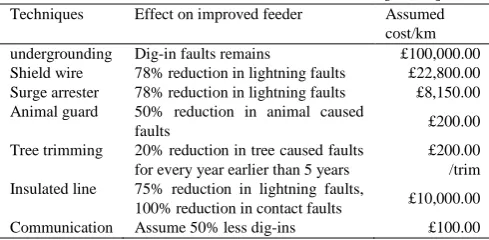
2) Network-based solutions: Voltage disturbance including voltage sags and interruption observed in distribution networks originate typically from short circuit faults in the transmission and distribution networks. Thus voltage disturbance of this type can be mitigated by reducing the possibility of fault occurrence. The mitigating solutions that can be implemented at critical locations (ones with higher fault rates) is provided in Table 1 [15, 16]. Instead of reducing fault rates, the phenomena of voltage sags can be also mitigated by reducing the fault severity. The severity of faults can be reduced by reducing fault clearing time, i.e., the response time of circuit breakers, or by placing fault current limiters around the network. Apart from filters, harmonics can also be mitigated by placement of line reactors [17], by the selection of appropriate transformer winding connections [2], using zigzag and grounding connected or transformers phase shifting transformers (quasi 12-pulse methods) [17].

Table 1

Effectiveness and cost of various network based solutions [15,16]

Techniques Effect on improved feeder Assumed cost/km undergrounding Dig-in faults remains £100,000.00 Shield wire 78% reduction in lightning faults £22,800.00 Surge arrester 78% reduction in lightning faults £8,150.00 Animal guard 50% reduction in animal caused

faults £200.00

Tree trimming 20% reduction in tree caused faults for every year earlier than 5 years

£200.00 /trim Insulated line 75% reduction in lightning faults,

100% reduction in contact faults £10,000.00 Communication Assume 50% less dig-ins £100.00

2.2. Financial Assessment

When financially assessing PQ mitigation at planning level, it is important to consider the benefits during the entire life span of the deployed solution. The upfront investment made for a mitigation solution pays back its returns only during the life span duration. This makes it important to consider the net present value of future benefits, as well as the net present value of future maintenance. This brings the investment cost and its future benefit to a common ground/level of comparison with planning or deployment year as the reference. The net present value approach accounts for the factors like inflation (denoted as i), discount rate (denoted as r) and escalation rate (denoted as e) required for the assessment of time value of money. Net present value (NPV) can be calculated using the following equation [14]:

𝑁𝑃𝑉 = 𝐶𝐼 +∑𝑛𝑡=0(𝐶𝑡𝑏+𝐶𝑡𝑐)×(1+𝑒)𝑡

((1+𝑟)(1+𝑖))𝑡 (1)

where CI denotes the initial capital investment (usually expressed as a negative amount), Ctb denotes the benefit

component (difference between original cost and remaining cost after the installation of the solution) occurring at the beginning of time period t; and Ctc

denotes the cost component (annual maintenance cost)

occurring at beginning of time period (usually expressed as a negative amount).

1) Assessment of financial consequence of PQ phenomena

Detailed analysis of economic impact due to voltage sags, unbalance and harmonics are very important while considering the investment in PQ mitigation. Economic impact can be assessed by identifying losses to different types of business due to various PQ phenomena. Considering the diversity of business types that exists, customers can be categorized based on their previous history of economic losses due to inadequate PQ performance, similarities in their business process and the sensitivity of their equipment/devices. This categorization enables the evaluation of the economic impact of a group of customers using a common model, thus each category has a unique model for analysis. This economic impact provides an estimate of financial losses for that particular customer at a given level of PQ in the network. Since losses caused by voltage sags, unbalance and harmonics are due to different reasons, it requires separate financial assessment models for each of them.

The financial losses to industrial customers due to voltage sags are mainly caused by the subsequent process trips. When assessing the probability of having process trips the main elements/parameters that should be considered include sag characteristics, frequency of sags at the customer busbars, equipment sensitivity, customer plant sensitivity, process operational cycle and the plant’s load profile [18]. With realistic modelling of process cycle and proper probabilistic modelling of uncertainties associated with each of the influential parameters, risk-based analysis approach is applied to assess the possibility of having industrial process trips by modeling the industrial process and performing risk analysis with the consideration of process immunity time [19]. The financial loss due to a sag event can be assessed by:

(Financial

loss ) = ( Process failure risk) × (Loss due to process trip) (2)

where the loss due to process trip can be obtained through survey or from customers directly.

According to the general classification of unbalance cost proposed by CIGRE/CIRED C4.107 report in the context of customers [9], economic losses due to unbalance phenomena are mainly caused by power and energy losses and the shortened life of equipment. NEMA recommends the use of de-rating curves for calculating power loss in induction motors [20]. The loss of power can be converted to financial cost using the rate of unit cost of energy over a period of time. By applying the NPV method it is possible to identify the accumulated cost of energy losses over the period of system study. These costs are considered as operating costs since this gets accounted into the operating expense incurred from payment of electricity charges by a business.

thermal stress can be modeled as [22, 23]:

𝐿 = 𝐿′0𝑒−(𝐵𝑐𝜃) (3)

where 𝐿′₀ refers to the reference life of the equipment for reference temperature 𝜃𝑜; B is a constant for a material

represented as B = E/K, where E is the activation energy of the aging reaction in Joule/mol and K is the gas constant in JK-1mol-1; 𝜃 is the operating temperature in the presence of unbalance.

As per NEMA guidelines the approximate increase in winding temperature ∆𝜃 in induction motors due to percentage voltage unbalance 𝑉_𝑎𝑠 can be calculated using ∆𝜃 = 2𝑉𝑎𝑠2 . A decrease in useful life of the motors results

in economic loss due to equipment replacement and process disruption caused by the equipment damage. The financial cost due to equipment ageing can be calculated to a good approximation by (𝐿′0− 𝐿)/𝐿′0× 𝐶𝑟𝑒, where 𝐶𝑟𝑒

denotes the cost of replacing the motors [9, 21].

Financial losses due to voltage/current harmonics can be classified into the categories of energy losses, losses due to premature ageing and losses due to equipment malfunction. CIGRE/CIRED C4.107 report suggests the methodologies for evaluating economic losses arising from wave form distortion caused by harmonics [9]. The losses in electrical motors caused by harmonics can be calculated with [9]:

𝑃𝑀= 3 ∑ (𝑉

ℎ 𝑍_𝑀ℎ)

2

𝑅𝑀ℎ ℎmax

ℎ=ℎ1 + 𝑃𝑐𝑜

1_{∑ (}𝑉ℎ 𝑍_𝑀ℎ)

𝑚𝑀 ₁ ℎ0.6 ℎmax

ℎ=ℎ1 (4)

where 𝑉ℎ represents the voltage harmonic of order h; 𝑍_𝑀ℎ and 𝑅_𝑀ℎ denote the equivalent impedance and resistance of the motor at the harmonic of order h respectively; 𝑃𝑐𝑜1

denotes the core loss at the fundamental frequency; and 𝑚𝑀 is the numerical coefficient.

Harmonic distortions also cause additional electric and thermal stresses in the insulating materials of electric equipment. A simple electro thermal life model recommended by CIGRE/CIRED C4.107 can be represented by [22, 23]:

𝐿 = 𝐿′0(𝐾𝑝) −𝑛_𝑝

𝑒−(𝐵𝑐𝜃) ₍₅₎

where 𝐾𝑝 is the peak factor of the voltage waveform,

represented by 𝐾_𝑝= 𝑉_𝑝/𝑉_1𝑝∗ where 𝑉_𝑝 is the value of the distorted voltage and 𝑉1𝑝∗ is the peak value of the

fundamental voltage; 𝑛𝑝 is the coefficient related to the

shape of the distorted waveform; 𝑐𝜃 = 1/𝜃0− 1/𝜃.

The aforementioned financial losses due to various PQ phenomena can be summed up and their NPV is calculated to identify the present worth of future economic PQ losses, by applying ∑𝑛𝑡=0𝐶𝑃𝑄𝑡× (1 + 𝑒)𝑡/((1 + 𝑟)(1 +

𝑖))𝑡where CPQt denotes the sum of costs due to different

PQ phenomena at time period t, and e, i and r are, as before, escalation rate, inflation and discount rate, respectively .

The assessed financial cost may vary in practical depending on the accuracy of the data collected from customers. Generally with more accurate information used for assessment, the financial analysis will provide more valuable reference. The data accuracy can be evaluated by the nature of customers and data source etc. If the cost information is not provided by certain customers, it can be estimated from customers with similar nature but assigned with larger uncertainty for probabilistic financial

assessment.

2) Financial assessment of mitigation techniques

The capital costs of SVC, DVR and PF can be obtained based on curve fitting approach using available cost records. The costs of DVR and STATCOM are considered to be the same. The capital cost including construction cost of these devices can be defined as [12]:

𝐶𝑆𝑇𝐴𝑇+𝐶𝑜𝑛= 553(−0.0008𝑆𝑆𝑇𝐴𝑇2 + 0.155𝑆𝑆𝑇𝐴𝑇+ 120) (_{𝑀𝑉𝐴𝑟}£ ) (6)

𝐶𝐷𝑉𝑅+𝐶𝑜𝑛= 553(−0.0008𝑆𝐷𝑉𝑅2 + 0.155𝑆𝐷𝑉𝑅+ 120) (_{𝑀𝑉𝐴𝑟}£ ) (7)

𝐶𝑆𝑉𝐶+𝐶𝑜𝑛= 553(0.0003𝑆𝑆𝑉𝐶2 − 0.3051𝑆𝑆𝑉𝐶+ 127.38) (_{𝑀𝑉𝐴𝑟}£ ) (8)

where 𝑆𝑆𝑇𝐴𝑇 , 𝑆𝐷𝑉𝑅 and 𝑆𝑆𝑉𝐶 denote the sizes of

STATCOM, DVR and SVC respectively. Continuous maintenance costs incurred every year during the life time are assumed to be 5% for SVC, and 10% for STATCOM and DVR, of their capital cost.

A conservative reactance of 0.1p.u. is used for each Fault Current Limiter (FCL), and the cost of owning and installing FCL is based on the cost model with the ten-year owning costs based on ABB products [24], with annual operation and maintenance costs at 5% of initial cost. The cost of passive filters is based on [25], with the continuous maintenance costs incurred every year assumed to be 5%. The cost of placing phase shifting transformers are based on [17], with annual maintenance costs at 5% of initial cost. The transformer connection related cost is calculated based on [26], assuming that the copper wire is 3% of the weight of the distribution transformers, and the weight of distribution transformers is based on ABB oil distribution transformer catalogue. The investment costs of other network-based mitigation techniques are given in Table 1, with annual maintenance costs at 5% of the initial cost. Tree trimming is scheduled to be carried out every 5 years.

2.3. Provision of Differentiated PQ levels

should be considered simultaneously when searching for the optimal mitigation solution. In this paper, Unified Bus Performance Index (UBPI) defined as (9) is adopted to represent the aggregated performance of the three PQ phenomena [3]:

𝑈𝐵𝑃𝐼𝑖,𝑗=AHP (𝐵𝑃𝐼𝑖,𝑗, 𝑇𝐻𝐷𝑖,𝑗, 𝑉𝑈𝐹𝑖,𝑗) (9)

where AHP (Analytic Hierarchy Process) is the aggregation procedure introduced in [27] and applied in [3] for assessment of aggregate PQ performance. With this aggregation approach, the gap between the actual PQ performance UBPI and the aggregated thresholds UBPITH

as given in (10) is adopted to reflect the customers’ satisfaction level on the PQ performance received.

𝑃𝑄𝐺𝐼UBPI= ∑ (∑ |𝑈𝐵𝑃𝐼𝑖,𝑗− 𝑈𝐵𝑃𝐼TH,𝑖|_UBPI

𝑖,𝑗>𝑈𝐵𝑃𝐼TH,𝑖 𝐵𝑖

𝑗=1 )

𝑁

𝑖=1

(10)

Further details regarding the aggregation index and the provision of differentiated PQ levels can be found in [3].

2.4. Problem Definition and Optimisation

In the study, the problem is defined as an optimisation problem, which applies the mitigation solutions in the network optimally in order to minimise the overall financial cost that includes the investment cost, operation/maintenance cost and the cost caused by various PQ phenomena, and to maximise the benefits as a result of the application of mitigation solution. Simultaneously, in planning PQ mitigation, the provision of differentiated PQ levels should be facilitated among different zones of the network based on customers’ requirements. The provision of differentiated PQ levels is considered as the technical requirement, and treated as a constraint to be imposed during the optimisation process. In the study, the technical requirement is included in the objective function using Lagrangian relaxation [28]. The present value of annual operation/maintenance cost and cost due to various PQ phenomena during the entire life span of the deployed solution is calculated using NPV method. To achieve the aforementioned objectives, an objective function (F) to be minimised in the optimisation problem is proposed and defined as:

𝐹 = 𝐶𝑚− 𝐶𝑏+ 𝛽 × 𝑃𝑄𝐺𝐼UBPI (11)

𝐶𝑚= 𝐶𝐼𝐶𝐼+

∑𝑛𝑡=0(𝐶𝐴𝑛𝑛𝑂𝑝𝑒𝑀𝑎𝑖𝑡 )×(1+𝑒)𝑡

((1+𝑟)(1+𝑖))𝑡 (12)

𝐶𝑏 = ∑ (𝐶𝑃𝑄

1𝑡_−𝐶 𝑃𝑄2𝑡)×(1+𝑒)𝑡 𝑛

𝑡=0

((1+𝑟)(1+𝑖))𝑡 (13)

where 𝐶_𝑃𝑄1𝑡 and 𝐶_𝑃𝑄2𝑡 denote the costs of PQ phenomena without and with mitigation, respectively at time period t

and 𝛽 is a Lagrange multiplier which imposes the penalty to the selected mitigation scheme if the technical constraints are violated. The total period for evaluation is 40 years. To avoid confusion, all cost variables in (11)-(13) are expressed as positive values (£). It can be seen that the smaller 𝐶𝑚 is, the less investment cost is required. The

financial benefit of placing the mitigation techniques, denoted as 𝐶𝑏, is calculated by (𝐶𝑃𝑄1𝑡− 𝐶𝑃𝑄2𝑡), as shown in

(13). In (11), negative sign is applied to 𝐶𝑏𝑒𝑛𝑒𝑓𝑖𝑡 so that the

optimisation procedure will attempt to maximise the benefit. 𝐶 = (𝐶𝑚− 𝐶𝑏) < 0 suggests that the subsequent

financial benefits resulting from the application of mitigation techniques will cover the initial capital

investment and maintenance cost of these mitigation techniques, and placing the selected mitigation scheme is beneficial in the long run.

2.5. Optimisation Methodology

In order to optimally place the mitigation techniques introduced in Section 2.1, potential and effective locations are selected based on evaluated PQ performance together with sensitivity analysis, and will be made initially available for optimisation search. Geography feasibility of the potential mitigation location should be also considered during selecting the potential mitigation techniques. Locations are selected based on rankings of buses, which are ranked based on BPI, VUF and THD, and the sensitivity of the voltages on the injection of reactive and

active power, i.e., ∑ |𝜕𝑉𝑗

𝜕𝑄| 𝑁_𝐵

𝑗=1 and ∑ |

𝜕𝑉_𝑗 𝜕𝑃| 𝑁_𝐵

𝑗=1 . With these

rankings, global and zonal selection of the potential locations are carried out based on the whole network and zonal information respectively [3]. Given the pool of pre-selected locations and the applied mitigation techniques, greedy algorithm is applied to find out the optimal mitigation solution (i.e., the optimal locations for the implementation of mitigation techniques and the optimal settings for the applied techniques if exist) to minimise the objective function F as defined in (11), which incorporates both financial assessment (including PQ cost and cost of PQ mitigation) introduced in Section 2.2 and technical requirement provided in Section 2.3. The search procedure in optimisation is terminated if either of the following requirements is met: 1) the number of iterations reaches the predefined maximum number; 2) the improvement of PQ performance between two continuous iterations is negligible by being smaller than a preset value.

3. Case Study

3.1. Test Network

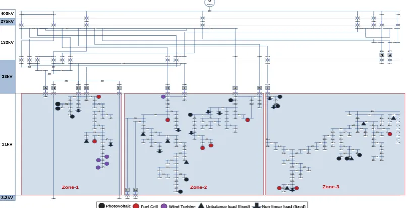
Fig. 1. Single line diagram of 295-bus generic distribution network.

of harmonic injection. The locations of the unbalanced loads, non-linear loads and different types of distributed generators are marked in Fig. 1. Based on the distribution of different classes of customers in certain area and the assumed PQ requirement of the predominated customers, the network is divided into three zones, as given in Fig. 1. The customers in zone 2 (predominately the industrial loads) have the most rigorous PQ requirement in the study, thus the UBPITH in this zone is set to 0.1724. To

present the different PQ requirements by customers in different zones, UBPITH in zones 1 and 3 are set to

0.2492and 0.4628 respectively [3]. In the study, the zone division given in Fig. 1 and zonal PQ requirement are set for illustrative purposes only. The BPI thresholds/limits in zones 1-3 are set to 0.8, 0.5 and 1.5 respectively; the THD thresholds are set to 0.5, 0.3 and 1 respectively; and the VUF thresholds are set to 1, 0.8 and 2 respectively. In total 500 sets of weights were adopted to calculate priorities among different PQ phenomena using AHP, and the ranges adopted to select weights for BPI, THD and VUF are [10, 20], [5, 15] and [6, 10], respectively. The average of the 500 obtained aggregated indices is then taken as the final aggregated index. Further details regarding the settings adopted to calculate UBPI can be found in [3] and [29]. The simulations related to the modellings of mitigation devices and various PQ phenomena are implemented in commercial software DIgSILENT/PowerFactory.

Different components are assigned with different fault rates based on the types of the components and their voltage levels. The assessment of voltage sags takes into account failure probability of primary protection relays and the uncertainty of the fault clearing time, which are generated randomly based on predefined normal distributions. Real power demand at each phase of the unbalance loads is set based on true load profiles. The reactive power of these unbalance loads is derived from randomly generated power factors which follow a normal distribution with the mean of 0.95 representing a general load. Among the 30 non-linear loads, 10 of them inject

harmonic current into the grid at fixed locations, named as fixed non-linear loads. The rest 20 non-linear sources are randomly selected from the unselected load buses and their location varies with operating condition. The modelling of harmonic current injection takes uncertainty into account by setting the ratio of the injected harmonic current to the fundamental component based on predefined normal distributions.

The variation of network parameters and load profiles are considered in the study in order to accurately evaluate the PQ performance. Annual hourly output curves of wind turbines and photovoltaic are extracted from realistic outputs data in UK [30, 31]. The outputs of fuel cells are assumed to be constant. The annual hourly loading information of various types of loads, including industrial, commercial and residential loads, are obtained from 2010 survey [32]. The maximum loadings of various types of customers and the maximum outputs of the wind turbine and photovoltaic are at different times of the year. In total 8760 operating points are obtained to present the annual operating condition. Though loadings of different types of loads (commercial, industrial and domestic loads) and the outputs of different types of DGs have their own variation patterns in terms of day and season, similar operating conditions repeat throughout a year. In the study, the annual operating points are clustered using Cluster Evaluation of Statistics Toolbox in Matlab, and the centroids of the clusters are selected as the representative operating conditions. The method of Silhouette is applied to evaluate the appropriateness of the obtained clusters. The study also take into account the extreme operating points, e.g., the operating condition corresponding to the maximum loadings of various types of loads (i.e., domestic, industrial and commercial loads) and the maximum outputs of various DGs (wind turbines and photovoltaic). In total 16 characteristic operating points are simulated in the study. The mean of the PQ performance evaluated from the 16 operating points respectively is used to calculate the aggregated PQ performance and incorporated in the objective function for 24 46 17 28 16 14 12 26 21 19 23 223 22 18 15 54 52 53 230 50 75 228 74 229 20 221 51 76 13 268 87 48 47 49 222 43 42 41 40 39 38 37 269 235 236 231 78 79 80 81 85 88 290 82 83 84 291 91 92 93 95 94 96 97 98 101 99 100 102 103 104 105 106 107 108 109 110 111 112 113 114 115 116 121 122 123 124 125 126 127 128 117 118 119 120 86 11 10 8 9 7 6 5 4 55 1 65 64 66 63 57 226 227 58 149 147 154 155

150 153 156

148 146 145 141 143 142 144 140 139 129 130 133 131 135 137 136 138 134 157 161 158 186 184 132 160 165 162 163 164 166 167 168 169 170 180 181 182 183 185 187 188 189 190 191 192 193 194 197 198 200 199 201 202 203 204 205 206 207 208 209 151 152 224 232 77 159 225 215 216 211 212 210 213 214 217 218 171 219 220 172 173 174 175 176 177 178 62 60 59 61 2 3 72 70 179 25 27 29 30 32 31 33 34 35 36 71 68 67 69 73 89 45 44 249 250 266 267 242 252 260 289 237 244 261 251

241 246 245 243

262 272 270

253 274

271 276 275 263 264 273

240

254

258 259 256

277 247 278 248 280 234 279 233 255 257 293 292

294 295 297 296

299 298 300 77 238 288 269

287 286 285

56

B

A C D E

F

H I J K L

O N G 132kV 33kV 11kV 3.3kV 275kV 400kV G 195 196

Zone-1 Zone-2 Zone-3

the purpose of optimisation. Table 2 provides the examples of the structure of industrial processes used for calculating the financial loss to industrial customers [10]. The nominal life of the motors used in the financial assessment is set to 40 years, and the nominal operating temperature is 85oC. The distribution of the causes of the faults in the network, i.e., lightning faults, animal contact, tree contact and dig-in faults etc., are based on [16].

Table 2

Details of Processes Adopted for Financial Assessment

Cust. Equipment Sub

Process

Process dependency Matrix

A PLC, ASD 1,2,3,4 1111,1101,1010,0111 B PLC, ASD 1,2,3,4 1111,1101,0010,0111 C PLC, ASD, Contactor 1,2,3,4 1111,1101,0010,1001

D PC, ASD 1,2,3,4 110,110,001

3.2. Simulation Results

In the study, the Lagrange multiplier 𝛽 in (11) is set in a way that the evaluated technical constraint component (𝛽 ×PQGIUBPI) is approximately equal to (or slightly

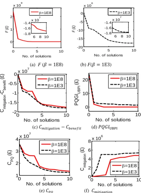
larger than) the costs of PQ phenomena. Based on this, 𝛽 is set to 1E8. The convergence curves of various variables, including F, 𝐶, 𝑃𝑄𝐺𝐼UBPI, 𝐶𝑚, and 𝐶𝑃𝑄 (i.e., the NPV

cost of PQ phenomena calculated over the life span of mitigation solution), are presented in Fig. 2.

(a) F (𝛽 = 1E8) (b) F(𝛽 = 1E3)

(c) 𝐶𝑚𝑖𝑡𝑖𝑔𝑎𝑡𝑖𝑜𝑛− 𝐶𝑏𝑒𝑛𝑒𝑓𝑖𝑡 (d) 𝑃𝑄𝐺𝐼UBPI

(e) 𝐶𝑃𝑄 (f) 𝐶𝑚𝑖𝑡𝑖𝑔𝑎𝑡𝑖𝑜𝑛

Fig. 2. Convergence curves of various components against the number of mitigation solutions applied.

Table 3

PQ Costs and Benefits Obtained Over the Lifetime of Devices and Pay Back Period

Case PQ cost Benefits Pay-back

(years) No mitigation £35,700,000.00 N/A N/A

β = 1E8 £13,400,000.00 £22,300,000.00 6

β = 1E3 £12,400,000.00 £23,300,000.00 5

Without mitigation, only the Lagrange component

𝛽 × 𝑃𝑄𝐺𝐼UBPI, i.e., the technical constraints of (UBPI

-UBPITH), contributes to the objective evaluation. At the

leftmost points in Fig. 2 (a), F=2.41E9 when 𝛽 = 1E8. It can be seen that the objective value F is reduced significantly after one solution is applied to the grid. When the number of mitigation solutions >5, F tends to converge steadily, though its improvement is not as significant as that when the number of mitigation solutions <5. As seen from (11), F is composed of 𝐶 and 𝛽 × 𝑃𝑄𝐺𝐼UBPI. The two components are presented in Fig.

2 (c) and (d), respectively. Without any mitigation, both 𝐶𝑚 and 𝐶𝑏 are zero. Thus it can be seen from Fig. 2 (c)

that 𝐶 = 0 when the number of solutions applied is zero. Afterwards, the obtained 𝐶 is smaller than zero constantly, which suggests that the financial benefits resulting from the application of the selected mitigation solution at the network level will cover the initial capital investment and maintenance cost of the mitigation. The costs of PQ phenomena and PQ mitigation are presented in Fig. 2 (e) and (f) respectively, and it can be seen that 𝐶𝑃𝑄 follows the same convergence trends as that in Fig. 2

(c). Table 3 provides the PQ related financial loss (without and with mitigation), the benefits over the lifetime of devices and the pay-back periods. The investment cost can be paid back within six years when 𝛽 = 1E8.

To present the PQ performance throughout the network visually, and for the convenience of comparing the aggregated UBPI obtained with and without mitigation, the heatmaps of UBPIs obtained without mitigation and with 10 devices (𝛽 = 1E8) are plotted in Fig. 3 (a) and (b) respectively. The critical area marked in red in Fig. 3 (a) is exposed to severe PQ disruption, and it is greatly improved by applying the optimal mitigation solution obtained, as shown in Fig. 3 (b).

(a) without mitigation

(b) with mitigation (𝛽 = 1E8 )

Fig. 3. Heatmaps of UBPIs obtained with the application of 10 solutions with and without mitigation.

0 5 10

0 1 2

x 109

No. of solutions

F

(£

)

0 5 10

-20 -15 -10 -5 0

x 106

No. of solutions

F

(£

)

6 8 10 -1.8 -1.6 -1.4x 10

7

6 8 10 -1.8 -1.6 -1.4x 10

7

=1E8 =1E3

0 5 10

-2 -1.5 -1 -0.5

0x 10

7

No. of solutions

Cm iti g a tio n -Cb e n e fit ( £ ) =1E8 =1E3

0 5 10

0 10 20

No. of solutions

P

Q

G

IUB

P

I

(

£

) =1E8

=1E3

0 5 10

1 2 3 4x 10

7

No. of solutions

CPQ ( £ ) =1E8 =1E3

0 5 10

0 2 4 6 8x 10

6

No. of solutions

Cm iti g a tio n ( £ ) =1E8 =1E3 149 147 154 155 150 153 156

148 146 145 141 143 142 144 140 139 129 130133 131 135 137136 138 134 157 161 158 186 184 132 160 165 162 163 164 166 167 168 169 170 180 181 182 183 185 187 188 189 190191 192 193 194 197 198 200199 201 202 203204 205 206 207 208 209 151 152 224 232 77 159 225 215 216 211 212 210 213 214 217 218171 219 220 172 173 174 175 176 177 178 265 195 196 L 24 46 17 28 16 14 12 26 2119 23 22322 18 15 54 52 53 230 50 75 228 74 229 20 221 51 76 13 268 87 48 47 49 222 43 42 41 40 39 38 37 269 231 78 79 80 81 85 88 290 82 83 84 291 91 92 93 95 94 96 97 98 10199 100 102 103104 105 106107 108 109 110 111 112 113 114115 116 121 122 123 124 125 126 127 128 117 118 119120 86 11 10 8 9 7 6 5 4 55 1 65 64 66 63 57 226 227 58 62 60 59 61 2 3 72 70 179 25 27 29 30 32 31 33 34 35 36 71 68 6769 73 89 45 44 266 267 289 238 288 269

287286285

56

B

A CD E H I J K

264 263 260 33kV 11kV 149 147 154 155 150 153 156

148 146 145 141 143 142 144 140 139 129 130133 131 135 137136 138 134 157 161 158 186 184 132 160 165 162 163 164 166 167 168 169 170 180 181 182 183 185 187 188 189 190191 192 193 194 197 198 200199 201 202 203204 205 206 207 208 209 151 152 224 232 77 159 225 215 216 211 212 210 213 214 217 218171 219 220 172 173 174 175 176 177 178 265 195 196 L 24 46 17 28 16 14 12 26 21 19 23 22322 18 15 54 52 53 230 50 75 228 74 229 20 221 5176 13 268 87 48 47 49 222 43 42 41 40 39 38 37 269 231 78 79 80 81 85 88 290 82 83 84 291 91 92 93 95 94 96 97 98 101 99 100 102 103104 105 106107 108 109 110 111 112 113 114115 116 121 122 123 124 125 126 127 128 117 118 119120 86 11 10 8 9 7 6 5 4 55 1 65 64 66 63 57 226 227 58 62 60 59 61 2 3 72 70 179 25 27 29 30 32 31 33 34 35 36 71 68 67 69 73 89 45 44 266 267 289 238 288 269

287286285

56

B

A C D E H I J K

264 263 260

33kV

11kV

The data provided by customers present different accuracy levels depending on data sources and customer nature. Industrial customers may have more sophisticated approaches to collect data and thus have more accurate cost information. In the simulation, customers are classified into three groups with each assigned with one of the uncertainty levels, i.e., 2.5%, 5% or 7.5% variation. The obtained solution is analysed and it gives that the standard deviation of the PQ cost obtained is 1.59E5, while that of the benefit is 1.83E5. The benefit is slightly larger than PQ cost as the uncertainty of the PQ cost without mitigation also contributes to the variation of the final benefit calculation. As for the economic assessment of the mitigation solutions, the capital investment cost and annual maintenance cost are also assigned different level of accuracy, namely 2.5% and 7.5% variation, respectively. The value of capital investment is assumed to be more accurate than the maintenance cost as the latter will occur in the future. The results yield 4.43% variation in the assessed total mitigation cost due to the assumed variation (inaccuracy) in capital and maintenance costs. At the same time the results show that the variation of the assumed capital investment cost is more critical than the variation of the maintenance cost, even though the latter was three times higher (7.5% compared to 2.5% variation), due to its much higher share (61.35%) of the total mitigation cost. In this simulation, the most likely cost is used in the process of selecting the mitigation solution.

1) Comparison on different settings of 𝛽

In the study, 𝛽 is also set to a much smaller value 1E3, i.e., 1x103, to present the impact of 𝛽 on the solution selection. The convergence of various components obtained by setting 𝛽 to 1E3 is shown in Fig. 2. In Fig. 2 (c), for each convergence curve, except for the leftmost points of the curves, 𝐶 obtained when 𝛽 = 1E3 is always slightly smaller than that obtained when 𝛽 = 1E8. However, in Fig. 2 (d), 𝑃𝑄𝐺𝐼UBPI obtained with 𝛽 = 1E3

is constantly larger than that obtained when 𝛽 = 1E8. It can be seen that when 𝛽 is set to 𝛽 = 1E8 , the optimisation will favour the mitigation schemes which are able to meet the technical constraints well and at the same time are financially preferable, especially at the early stage of the optimisation process. From a financial perspective the mitigation cost can be paid back one year earlier when 𝛽=1E3 compared to the case of = 1E8 as seen from Table 3.

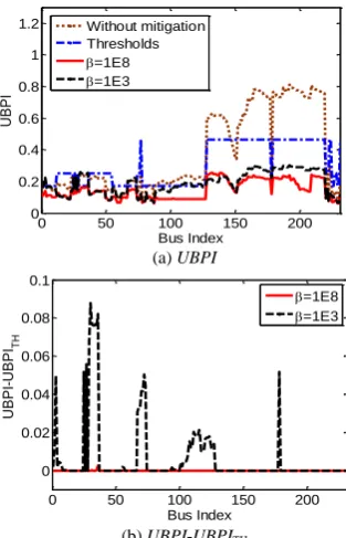
With smaller 𝛽, the importance of technical constraints are not addressed as well as when 𝛽 = 1E8, as shown in Fig. 2(d). The satisfaction of the received PQ performance in comparison to customer specified thresholds, UBPIs evaluated at all buses together with the specified thresholds are provided in Fig. 4 (a). It can be seen that without mitigation, most buses violate the PQ thresholds. With the application of the mitigation solution obtained with 𝛽 = 1E8, the PQ performance received at almost all buses meet the corresponding PQ thresholds. If the mitigation solution obtained with 𝛽 = 1E3 is applied to the grid, there still exit a relatively large number of UBPIs which are larger than the PQ thresholds. To present the gap between the received UBPIs and the thresholds, (UBPI

-UBPITH) evaluated at all buses are also given in Fig. 4 (b).

With 𝛽 = 1E8 , the technical constraints are met

stringently. However, when 𝛽 = 1E3, in total there are 64 buses violating the requirements.

The solutions obtained for 𝛽 = 1E3 and 𝛽 = 1E8 respectivelyare listed in Table 4 including the type, size and installation location of the selected FACTS devices and the zones of the selected network-based techniques. The network-based solutions which can be implemented at critical locations in zones are selected, in both cases, based on to their cost-effectiveness advantage. When 𝛽 = 1E8 (see Table 4) the obtained optimal solutions consist of three FCLs that contribute to the mitigation of fault severity and when 𝛽 = 1E3 the obtained solution consists of three phase shift transformers that contribute to the harmonic mitigation. When 𝛽 = 1E3, apart from the sag mitigation, harmonic mitigation is emphasized as well due to the financial cost caused by this phenomenon. It can be seen that the influence of the PQ phenomena on the final mitigation solution varies depending on their contribution to economic and technical evaluations.

(a) UBPI

(b) UBPI-UBPITH

Fig. 4. PQ performance of various buses obtained with 10 solutions.

Table 4

Optimal Solutions for Different PQ Phenomena

PQ type (size MVA) and location of mitigating solutions

𝛽 = 1E3 DVR (4.73) at B82; PF (2.18) at B135; phase shifting transformer installation at B2, B86 and B100; cable communication improvement at critical locations in zones 2 and 3; animal guard at critical locations in zone 3; tree trimming at critical locations in zone 3; line insulation at critical locations in zone 3

𝛽 = 1E8 STATCOM (5.47) at B29; SVC (2.66) at B201; DVR (6.01) at B291; FCL at B47-B222; FCL at B153-B155; FCL at B211-B216; cable communication improvement at critical locations in zones 2 and 3; tree trimming at critical locations in zone 3; line insulation at critical locations in zone 3

Tech only

STATCOM (5.47) at B29; SVC (7.85) at B27; SVC (2.66) at B39; DVR (6.79) at B66; Animal guard at critical locations in zone 2

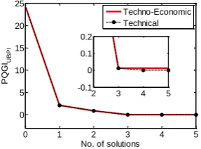
2) Comparison from technical performance index only

The optimisation based on technical performance index only is also carried out in the study. In total nine alternative mitigation strategies which meet PQGIUBPI=0

are obtained in the simulation. In this case one strategy

0 50 100 150 200

0 0.2 0.4 0.6 0.8 1 1.2

Bus Index

U

B

P

I

Without mitigation Thresholds

=1E8

=1E3

0 50 100 150 200

0 0.02 0.04 0.06 0.08 0.1

Bus Index

U

B

P

I-U

B

P

ITH

should be selected. The one with the least cost is selected (see Table 4). The convergence of its performance is shown in Fig. 5, together with that obtained from previous techno-economic analysis. It can be seen that the two approaches produce very similar technical convergence characteristic. However the technical index based approach is likely to choose device-based solutions which are more expensive as shown in Table 4.

Fig. 5. The comparison between two different analysis approaches.

4. Conclusions

The paper presents an optimisation-based methodology for global techno-economic PQ mitigation in distribution networks with renewable generation. It considers for the first time in published literature: i) Financial losses due to industrial process trips, equipment aging issues and power losses, etc. caused by several PQ phenomena simultaneously; ii)The cost of versatile mitigation solutions (including network-based and device-based mitigation solutions) over the entire life span of the deployed solution; iii) The provision of differentiated PQ levels to customers in different zones based on different zonal requirements by incorporating the technical requirements in the optimisation process using the approach of Lagrangian relaxation.

The simulation results illustrated using heatmaps of distribution network based on UBPIs, demonstrate that applying chosen mitigation solution is beneficial in the long run, as the financial benefits of applying the solution are much larger than the initial capital investment and maintenance cost of the PQ mitigation. The impact of the setting of Lagrangian multiplier 𝛽 on the final selected mitigation solution is also analysed. The results show that a larger 𝛽 allows the technical PQ requirements (minimizing the violation of set thresholds for considered PQ phenomena) to have more influence on the selection of the final solution, and smaller 𝛽 places more influence on the final cost of the solution, i.e., payback period.

Acknowledgments

This work was supported by SuSTAINABLE Project [Grant numbers 308755].

References

[1] Spec. Semicon. Process, Equipment Voltage Sag Immunity, SEMI-F47-0706. Available: www. Semi.org.

[2] R. Dugan, M. F. McGranaghan, S. Santoso, and H. W. Beaty,

Electrical Power Systems Quality (2 Ed.). New York: McGraw-Hill, 2002.

[3] H. Liao, S. Abdelrahman, and J. Milanovic, "Zonal Mitigation of Power Quality Using FACTS Devices for Provision of Differentiated Quality of Electricity Supply in Networks with Renewable Generation" IEEE Trans. on Power Deliv., vol. 32, no. 4, pp. 1975-1985, 2017.

[4] H. Masdi, N. Mariun, S. Mahmud, et. al, "Design of a prototype D-STATCOM for voltage sag mitigation," in Proc. National Power and Energy Conf., Kuala Lumpur, Malaysia, 2004, pp. 61-66. [5] J. V. Milanović and Y. Zhang, "Modeling of FACTS devices for

voltage sag mitigation studies in large power systems," IEEE Trans. Power Deliv., vol. 25, pp. 3044-3052, 2010.

[6] Y. Zhang and J. V. Milanović, "Global voltage sag mitigation with FACTS-based devices," IEEE Trans. Power Deliv., vol. 25, pp. 2842-2850, 2010.

[7] M. M. El Metwally, A. A. El Emary, F. M. El Bendary, and M. I. Mosaad, "Using FACTS controllers to balance distribution systems based ANN," in Proc. Int. Mid. East Power Syst. Conf., 2006, pp. 81-86.

[8] R. Grunbaum, "FACTS for voltage control and power quality improvement in distribution grids," in Proc. CIRED Semi. Smart Grids for Distrib., 2008, pp. 1-4.

[9] J. G. Lglesias etc., "Economic framework for power quality, JWG CIGRE-CIRED C4.107," 2011.

[10] J. Y. Chan, J. V. Milanović, and A. Delahunty, "Risk-based assessment of financial losses due to voltage sag," IEEE Trans. Power Deliv., vol. 26, pp. 492-500, 2011.

[11] J. V. Milanović and C. P. Gupta, "Probabilistic assessment of financial losses due to interruptions and voltage sags-part I: the methodology," IEEE Trans. Power Deliv., vol. 21, pp. 918-924, 2006.

[12] J. V. Milanović and Z. Yan, "Global minimization of financial losses due to voltage sags with FACTS based devices," IEEE Trans. on Power Deliv., vol. 25, pp. 298-306, 2010.

[13] F. B. Alhasawi and J. V. Milanović, "Techno-economic contribution of FACTS devices to the operation of power systems with high level of wind power integration," IEEE Trans. Power Syst., vol. 27, pp. 1414-1421, 2012.

[14] A. A. Groppelli and E. Nikbakht, Finance, Barrons Educational Series Inc, 2000.

[15] T. A. Short, Electric Power Distribution Handbook (2nd _edition).

New York: CRC Press, 2014.

[16] J. Y. Chan, "Framework for assessment of economic feasibility of voltage sag mitigation solutions," Ph.D., Ph.D. dissertation, Dep. Electr. And Electro. Eng., University of Manchester, Manchester, U.K., 2010.

[17] T. C. Sekar and B. J. Rabi, "A review and study of harmonic mitigation techniques," in Proc. Int. Emer. Trends in Elec. Eng. and Ener. Manag., Chennai, 2012.

[18] H. L. Liao, S. Abdelrahman, Y. Guo, and J. V. Milanović, "Identification of weak areas of power network based on exposure to voltage sags—Part II: assessment of network performance using sag severity index," IEEE Trans. Power Deliv. , vol. 30, pp. 2401 - 2409, 2015.

[19] J. C. Cebrian, J. V. Milanovic, and N. Kagan, "Probabilistic Assessment of Financial Losses in Distribution Network Due to Fault-Induced Process Interruptions Considering Process Immunity Time," IEEE Trans. Power Del., vol. 30, pp. 1478-1486, 2015. [20] N. E. M. Association, "NEMA Standards Publication MG 1-1998

Motors and Generators," ed, 2002.

[21] "Statistical classification of economic activities in the European Community," European Commission Eurostat, 2008.

[22] P. Caramia, G. Carpinelli, P. Verde, G. Mazzanti, A. Cavallini, and G. C. Montanari, "An approach to life estimation of electrical plant components in the presence of harmonic distortion," in Proc. 9th Int. Conf. on Harm. and Quality of Power, 2000, pp. 887-892 vol.3. [23] G. C. Montanari and L. Simoni, "Aging phenomenology and

modeling," IEEE Trans. Elec. Insul., vol. 28, pp. 755-776, 1993. [24] A. Cali, S. Conti, F. Santonoceto, and G. Tina, "Benefits assessment

of fault current limiters in a refinery power plant: a case study," in

Proc. Int. Conf. Power System Tech., 2000, pp. 1505-1510 vol.3. [25] M. Ghiasi, V. Rashtchi, and S. H. Hoseini, "Optimum location and

sizing of passive filters in distribution networks using genetic algorithm," in Proc. Int. Conf. on Emer. Tech., 2008, pp. 162-166. [26] M. Mohan, "Amorphous-Core Transformer with Copper Winding

Versus Aluminium Winding-A Comparative Study," ARPN Journal of Science and Technology, vol. 2, pp. 297-301, 2012.

[27] S. Abdelrahman, H. Liao, T. Guo, Y. Guo, and J. V. Milanović, "Global assessment of power quality performance of networks using the analytic hierarchy process model," in Proc. IEEE PowerTech, Eindhoven, 2015, pp. 1-6.

0 1 2 3 4 5

0 5 10 15 20 25

No. of solutions

P

Q

G

IUB

P

I

Techno-Economic Technical

2 3 4 5

[28] H. Everett, "Generalized Lagrange multiplier method for solving problems of optimum allocation of resources," Oper. Res., vol. 11, pp. 399-417, 1963.

[29] J. V. Milanović, Sami Abdelrahman and H. Liao, "Compound Index for Power Quality Evaluation and Benchmarking," IET Gen., Trans. and Distri., DOI: 10.1049/iet-gtd.2018.5391.

[30] CM SAF JRC EUROPEAN COMMISSION. Photovoltaic Geographical Information System - Interactive Maps [Online]. Available: http://re.jrc.ec.europa.eu/pvgis/apps4/pvest.php. [31] "The Renewable Energy Review," Committee on Climate Change,

2011.