A methodology for speeding up loop kernels by exploiting the software information and the memory architecture

A methodology for speeding up loop kernels by exploiting

the software information and the memory architecture

KELEFOURAS, Vasileios <http://orcid.org/0000-0001-9591-913X>,

KRITIKAKOU, Angeliki and GOUTIS, Costas

Available from Sheffield Hallam University Research Archive (SHURA) at:

http://shura.shu.ac.uk/18360/

This document is the author deposited version. You are advised to consult the publisher's version if you wish to cite from it.

Published version

KELEFOURAS, Vasileios, KRITIKAKOU, Angeliki and GOUTIS, Costas (2015). A methodology for speeding up loop kernels by exploiting the software information and the memory architecture. Computer Languages Systems and Structures, 41, 21-41.

Copyright and re-use policy

See http://shura.shu.ac.uk/information.html

A methodology for speeding up loop kernels by

exploiting the software information and the memory

architecture

Vasilios Kelefourasa

, Angeliki Kritikakoub

, Costas Goutisa

a

Department of Electrical and Computer Engineering, University of Patras ([email protected])

b

Education and Research Department in Computer Science and Electrical Engineering, University of Rennes 1

Abstract

It is well-known that today’s compilers and state of the art libraries have three major drawbacks. First, the compiler sub-problems are optimized separately; this is not efficient because the separate sub-problems optimization gives a different schedule for each sub-problem and these schedules cannot coexist as the refining of one, causes the degradation of another. Second, they take into account only part of the specific algorithms information. Third, they take into account only a few hardware architecture parameters. These approaches cannot give an optimumal solution.

In this paper, a new methodology/pre-compiler is introduced, which speeds up loop kernels, by overcoming the above problems. This methodology solves four of the major scheduling sub-problems, together as one problem and not separately; these are the sub-problems of finding the schedules with the minimum numbers of i) L1 data cache accesses, ii) L2 data cache accesses, iii) main memory data accesses, iv) addressing instructions. First, the ex-ploration space (possible solutions) is found according to the algorithm’s information, e.g. array subscripts. Then, the exploration space is decreased by orders of magnitude, by applying constraint propagation to the software and hardware parameters.

compilers and also with iterative compilation.

Keywords: Data reuse, register allocation, optimization, memory

hierarchy, loop tiling, data locality, Diophantine equations

1. Introduction

Regarding data dominant applications (for example linear algebra, im-age, signal and video processing algorithms), the major performance critical parameters are i) the number of main memory accesses, ii) the number of L3/L2 cache accesses, iii) the number of L1 data cache accesses and iv) the number of executed instructions (we assume that the number of the algorithm instructions cannot be reduced and thus we reduce only the number of addressing instructions). The above compilation/scheduling sub-problems are interdependent and thus they cannot be optimized separately; actually, the refining of one sub-problem causes the degradation of another, e.g. a decrease of the number of L2 data cache accesses will consequently increase the number of L1 data cache accesses. Researchers try to solve this problem by using iterative compilation techniques.

Iterative compilation has five major drawbacks, i) there are memory efficient schedules which cannot be produced by applying the existing com-piler transformations, ii) iterative compilation does not use all the existing transformations, including all the different transformation parameters, e.g. unroll factor values and tile sizes, because in this case compilation will last for years, iii) only one level of tiling is applied, which is not efficient, iv) register allocation is applied without taking into account the data reuse; this means that the arrays references are assigned into registers, without taking into account that some are accessed a lot and others do not, v) the data array layouts are not taken into account; we will show that when tiling to multidimensional arrays is applied, the data array layouts must change. These drawbacks are overcome by the proposed methodology.

array reference is given by its subscript equation. Given that the memory access pattern of each array is given by its subscript equation, we claim that all memory efficient solutions (exploration space) can be produced by processing these equations. The subscript equations are processed and a new iteration space is created. Each subscript equation gives either its iterators or even new iterators, to the new iteration space. Then, the exploration space is orders of magnitude decreased by applying constraint propagation to the software and hardware parameters. Regarding the hardware parameters, we produce register file and data cache inequalities, which contain all the (near)-optimum tile sizes; these inequalities contain i) the tiles sizes in elements, ii) the shape of each array’s tile. Furthermore, new data array layouts are generated, according to the data cache associativity. All the schedules with different tile sizes and data array layouts, than these the proposed methodology gives, are not considered, decreasing the exploration space.

The major contributions of this paper are: i) the optimization of the above subproblems as one problem and not separately for a wide range of algorithms and computer architectures, ii) the software information and several hardware parameters are fully exploited giving high execution speed solutions and a smaller search space, iii) the proposed methodology, due to the major contribution of number (ii) above, gives a smaller code size and a smaller compilation time, as it does not test a large number of alternative schedules, as the state of the art (SOA) libraries and iterative compilation do.

The experimental results are taken by using a general purpose proces-sor, an embedded processor and Simplescalar simulator [1]. The proposed methodology is evaluated for five well-known data dominant algorithms over two different compilers (speedup from 1.8 up to 18.3) and iterative compila-tion technique (speedup up to 2.2).

The remainder of this paper is organized as follows. In Section 2, the related work is given. The proposed methodology is given in Section 3 while the experimental results are given in Section 4. Finally, Section 5 is dedicated to conclusions.

2. Related Work

be optimized together as one problem and not separately. Toward this, much research has been done, either to simultaneously optimize only two phases, e.g. register allocation and instruction scheduling [2] [3] or to apply predictive heuristics [4] [5]. Nowadays compilers and related works, apply i) iterative compilation techniques [6] [7] [8] [9], ii) both iterative compilation and ma-chine learning compilation techniques to restrict the configurations’ search space and thus to decrease the compilation time [10] [11] [12] [13] [14] [15], iii) iterative optimizations or compiler transformations, by using the Polyhedral model [16] [17] [18] [19], iv) compiler transformations by using heuristics and empirical methods [20]. In iterative compilation, a large number of different versions of the program are generated-executed by applying many compiler transformations, at all different combinations. Iterative compilation requires extremely long compilation times to decrease the exploration space iterative compilation is applied with machine learning compilation techniques. The five major iterative compilation drawbacks are referred to the introduction. The proposed methodology achieves up to 2.1 times lower execution time and an orders of magnitude lower compilation time (Section 4).

The state of the art software libraries, such as ATLAS [21], GotoBLAS2 [22], Eigen [23], Intel MKL [24], PHiPAC [25], FFTW [26], OpenCV [27] and SPIRAL [28], manage to find a near-optimum binary code for a specific application by using a large exploration space (many different executables are tested and the fastest is picked). Although they achieve high speed, they are application specific and the final schedule is found mostly by using heuristics and empirical techniques. A comparison with the above libraries would be unfair because they use the SIMD (Single Instruction Multiple Data) vector instructions (they support load/store and arithmetical instruc-tions with 128/256-bit data); however, our future work includes the support of SIMD instructions. In [29] [30] [31] [32], we have developed algorithm specific methodologies (we used the SIMD instructions), which produce lower execution time, lower compilation time and lower number of data accesses, than ATLAS [29] [30], FFTW [30] and OpenCV [32]. A comparison between the proposed methodology and [29] [30], is made in Section 4.

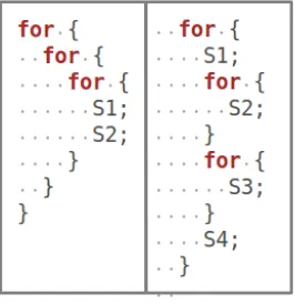
Figure 1: Perfectly and imperfectly nested loops are shown at (a) and (b), respectively.

Regarding register allocation problem, many methodologies exist such as [48] [49] [50] [51] [52] [53] [54]. In [48] - [52], data reuse is not taken into account; this means that the array references are assigned into registers, without taking into account that some are accessed a lot and others do not. In [53] and [54], data reuse is taken into account either by greedily assigning the available registers to the data array references or by applying loop unroll transformation to expose reuse and opportunities for maximizing parallelism. In contrast to the proposed methodology, the [48] - [54] address the register allocation problem without taking into account the scheduling problem; instead of finding a good schedule that achieves data reuse and then apply register allocation, they just apply register allocation to the given schedule.

3. Proposed Methodology

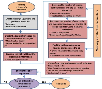
Create subscript Equations and put them into a list

Data reuse

Production-consumption

Create the Exploration Space (ES)

Data dependencies are satisfied

Many Iteration Spaces

Nesting level values are not defined yet

Decrease the number of data cache and main memory, accesses and the ES

- utilize the Data Cache memories parameters

Create DC inequalities

Create schedules utilizing the DC sizes

Find the optimum data array layouts and decrease the ES Create schedules with new data array layouts

Utilize the data cache associativities

Create final code and enumerate all solutions

Create final C-codes

Final C-codes are compiled by the target compiler The binaries run at the target architecture Best schedule is found

Decrease the number of L1 data cache accesses and the ES - utilize

the RF size Create RF inequalities

Create schedules utilizing the RF size

Decrease the ES by utilizing the algorithm’s information Fixed nesting level values

Parsing

Extract s/w information

Final Code Shuffle the list of

equations

Are all different list combinations processed ? M em or y a rc hi te ct ur e p ar am et er s Yes No

Figure 2: Flow graph of the proposed methodology.

The proposed methodology optimizes source code which contains loops (loop kernels); as it is well known, 90% of the execution time of a com-puter program is spent executing 10% of the code (also known as the 90/10 law) [55]. We take a loop kernel as input and we produce a new loop kernel which cannot be given by applying the existing transformations to the original code. The methodology optimizes both perfectly and imperfectly nested loops (Fig. 1), which i) no if-condition exists (if they do, current expression is skipped), ii) all the array subscripts are linear equations of the iterators (which in most cases do). Each loop kernel is optimized separately; each loop kernel may contain either perfectly or imperfectly nested loops (Fig. 1).

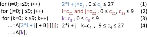
for (i=0; i≤9; i++)

for j=0; j ≤9; j++ for k=0; k ≤9; k++

...=A[2*i + j] + B[i][j]; ...=A[k];

2*i + j=c₁, 0 ≤ c₁≤ 27 (1)

i=c₂₁and j=c₂₂, 0 ≤ c₂₁, c₂₂ ≤ 9 (2)

k=c₃, 0 ≤ c₃≤ 9 (3) 2*i + j - k=c₄ , -9 ≤ c₄≤ 27 (4)

Figure 3: The three first equations contain the separate data reuse of the three array references respectively, while the fourth equation contains the data reuse between the two different references of the array A.

the data dependences, the subscript equations etc, are identified. Then, one mathematical equation is created for each array’s subscript and one for each two common array references (e.g. eq.(4) in Fig. 3, it is explained in Subsect. 3.3); each equation defines the memory access pattern of the specific array reference; data reuse is found by these equations. Given that the memory access pattern of each array is given by its subscript equation, we claim that all memory efficient solutions can be produced by processing these equations (Subsect.3.2). After all the equations have been created, all the equations are processed one by one, at all different combinations (Fig. 2), to examine all possible solutions (Subsect.3.2).

For each different combination (e.g. eq.(3), eq.(2), eq.(1) and eq.(4), in Fig. 3), all the equations are processed one by one, creating the new iteration space (Subsect. 3.4); the iteration space is defined by the iterators used and their nesting level values. Each equation inserts its iterators or even new iterators into the new iteration space; for an iteration space to be created all the equations must be fetched.

the layouts an additional cost is added which may degrade performance. All the schedules with different tile sizes and data array layouts than these the proposed methodology gives, are not considered, decreasing the exploration space. Finally, all these schedules are transformed into C-code, they are compiled by the target compiler and the output binaries are run to the target platform in order to find the one with the best performance (Subsect. 3.9).

The remainder of the proposed methodology has been divided into ten sub-sections. The first subsection contains the basic definitions and no-tations. The second presents a new loop transformation and the other seven ones explain in more detail the most complex steps of the proposed methodology (Fig 2). Finally the tenth subsection gives an example.

3.1. Definitions and Notations

Definition 1. Equations which have more than one solutions for at least one constant value, are named type2 equations. All others, are named type1 equations, e.g. eq.(1) and eq.(4) in Fig. 3 are type2 equations, while eq.(2) and eq.(3) are type1 equations.

Arrays with type2 equations fetch their elements more than once, even if no other/extra iterator exists (the loop kernel contains only the type2 equation iterators), e.g. 2i+j = 7 holds for several iteration vectors (data reuse); on the other hand, if no extra iterator exists, arrays with type1 equations fetch their elements only once. However, both type1 and type2 arrays may fetch their elements more than once because of the existence of another loop iterator(s) above/between from/of theirs; for example, although eq.(3) in Fig. 3 is of type1, each element ofA[k] is fetched 100 times because of the presence of i, j iterators.

To sum up, arrays with type2 equations achieve data reuse at all cases, while arrays with type1 equations achieve data reuse only at the case that extra iterators exist.

The arrays are classified into category-1 and category-2 arrays.

Definition 2. The arrays whose elements achieve data reuse are classified into category-1 arrays

Definition 4. The arrays whose subscript equations are of type1 and they contain all the loop kernel iterators (no extra iterator exists), are further classified into Category-2a arrays.

Statement 1. The Category-2a arrays fetch their elements just once (there is no data reuse).

Proof 1. The subscript equations of these arrays change their values in each iteration vector and thus a different element is fetched in each iteration.

Definition 5. The arrays whose subscript equations are not given by a com-pile time known expression (e.g. they depend on the input data), are further classified into Category-2b arrays.

Statement 2. Data reuse of Category-2b arrays cannot be exploited, as the arrays elements are not accessed according to a mathematical formula.

Definition 6. If all the iterators of an equation, exist in this equation only and not in another equation, then these iterators are named unique iterators, e.g. the i, j iterators of eq.(1) in Fig. 7 are unique, while the i, j iterators of eq.(1) in Fig. 3 are not.

3.2. Proposed Loop Transformation

As it has been explained in the previous subsection, arrays with type2 equations fetch their elements more than once (data reuse), even if no extra iterator exists. For example, the iteration vectors (S = (i, j, k)) fetchingA[4] of eq.(1) in Fig. 3, are more than one (data reuse), i.e. 2∗i+j = 4 holds for S1 = (0,4, X),S2 = (1,2, X) andS3 = (2,0, X), whereX are all the validk values. In this subsection, we propose a new loop transformation in order to exploit the data reuse of type2 equations. The new transformation treats the type2 equation as a Linear Diophantine Equation (LDE); the solution of an LDE is a mathematical expression which gives the exact iteration vectors that each array’s element is fetched only once, e.g. if the proposed transformation is applied on 2∗i+j =c1 of Fig. 3, each element ofA[2∗i+j] is accessed only once.

Proof 2. The minimum number of data accesses is achieved because each array’s element is accessed only once.

The proposed transformation can be applied only if there are no loop carried data dependencies.

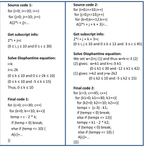
Let us give two examples, Fig. 4. The equation produced by the array subscript, gives all the information needed about the data reuse of array A. This equation is treated as a LDE here; its solution gives thei, j values that c is a constant value, e.g. c = 10 for all 0 ≤ k ≤10 values giving a j value within its bounds (source code 1 in Fig. 4). The solution of the Diophantine equation and the iterator bounds, give a new iteration space which all the array elements are fetched just once; i and j iterators are replaced by k and c iterators. To transform these equations into source code, a new iterator is added into the source code (c iterator) for all the array elements to be accessed in order. The added if-condition statements are necessary. In general, one if-condition statement is needed for each iterator, e.g. at source code 1, if-condition statements for both i and j iterators are needed; however, in most cases it is not necessary to add an if-condition statement for all the iterators because the Diophantine independent variable equals to the iterator, e.g. i=k in source code 1. Thus, the iterator bounds are preserved by the loop bounds and no if-condition statement is needed. The break statements have been inserted to decrease the number of idle iteration vectors.

If the proposed transformation is applied, the number of data accesses is minimized and the data cache lines utilization is increased since all the array’s elements are fetched in order and thus from consecutive memory locations. However, the number of arithmetical instructions is increased (extra addressing and branch instructions). The schedule with the minimum number of data accesses does not always provide the best performance, since the number of extra instructions may degrade performance; the best performance depends on the target architecture. This is why type2 equations are treated both as LDE equations and not. The two codes in Fig. 4 are the schedules with the minimum number of data accesses.

3.3. Create Equations

At this step, each array’s subscript is transformed into a mathematical equation (Fig. 3).

Source code 1:

for (i=0; i<=10; i++) for (j=0; j<=10; j++)

A[2*i + j]=...

Get subscript info:

2*i + j=c

0 ≤ i, j ≤ 0 and 0 ≤ c ≤ 0

Solve Diophantine equation:

i=k J=c-2k

0 ≤ k ≤ 0 and 0 ≤ c-k ≤ 0

0 ≤ k ≤ 0 and -5 ≤ k ≤ 5

Thus, 0 ≤ k ≤ 0

Final code 1:

for (c=0; c<=30; c++) for (k=0; k<=10; k++){

temp = c - 2 * k; if (temp < 0) break; else if (temp <= 10) { A[c]=...

}}

Source code 2:

for (i=0;i<=10;i++) for (j=0;j<=10;j++)

for (k=0;k<=12;k++) A[2*i + j + k + 3]=...

Get subscript info:

2*i + j + k + 3=c

0 ≤ i, j ≤ 0 and 0 ≤ k ≤ and ≤ c ≤ 5

Solve Diophantine equation:

We set w=2i+j (1) and thus w+k=c-3 (2) (2) gives: w=k1 and k=c-3-k1

0 ≤ k ≤ 0 and - ≤ k ≤

(1) gives: i=k2 and j=w-2k2

0 ≤ k ≤ 0 and -5 ≤ k ≤ 5

Final code 2:

for (c=3; c<=45; c++) for (k1=0; k1<=30; k1++){

for (k2=0; k2<=10; k2++){ tempz = (c-3) - k1; if (tempz < 0) break; else if (tempz <= 12){ tempy = k1 - 2 * k2;

if (tempy < 0) break; else if (tempy <= 10) { A[c]=...

}}}}

It is obvious that the memory access pattern of each array reference is given by its subscript equation.

Statement 5. The interaction of two or more equations gives i) the data reuse produced between the common array references (e.g. eq.(4) in Fig. 3) and ii) the interaction among the arrays data, i.e. by fetching one array’s element, other array elements are consequently fetched.

Regarding (i), in the case that there are two array references of the same array, an additional equation is always created to give the iteration vectors that both references access identical elements, e.g in Fig. 3, A[2] is fetched by S1=(0,2,X) and S2=(1,0,X) according to eq.(1) and also A[2] is fetched by S3=(X,X,2) according to eq.(3), where X = [0,9]. Regarding (ii), it is obvious that by fetching one array’s element, other array elements are consequently fetched, e.g. by fetching B(2,3) in Fig. 3, A(7) and A(0 : 9) are fetched because of the first and the second array reference respectively.

Rule 1. If there are two array references of the same array, an additional equation is created to describe the data reuse between these two references, e.g. eq.(4) in Fig. 3. These equations are further classified into type3 equations.

Rule 2. Regarding 2-d arrays, two equations are created and not one because the data array layout has not been found yet, e.g. if 9∗i+j = c2 is taken instead of i =c21 and j = c22 for eq.(2) in Fig. 3, then row-wise layout is taken which may not be efficient.

The Type1, type2 and type3 equations, are treated differently (Subsec-tions 3.3.1- 3.3.3).

3.3.1. Type1 equations

All type1 equations add their iterators into the new iteration space (their nesting level values are found next), e.g. eq.(2) of Fig. 3, gives either S1 = (i, j) iteration space or S2 = (j, i).

3.3.2. Type2 equations

reuse), e.g. if the proposed transformation is applied on 2∗i+j = c1 of Fig. 3, each element ofA[2∗i+j] is accessed only once. Type2 equations are treated in two different ways because the optimum data reuse of one array does not always provide the optimum data reuse or the best performance.

Rule 3. type1 equations give their iterators into iteration space, while type2 equations give either their iterators (they are treated as type1 equations) or new ones (the proposed transformation is applied, Statement 3), into iteration space.

3.3.3. Type3 equations

Type3 equations contain the iteration vectors that both two array ref-erences fetch the identical elements (data reuse), e.g. A[2] is accessed by (0,2, X) and (1,1, X) because of the A[i+j] reference and by (X, X,2) be-cause of theA[k] reference in Fig.2. This kind of data reuse is fully exploited too, by treating the type3 equations as LDE. Let us give an example, Fig. 5. The equation giving the iteration vectors that both two references fetch the identical array elements, is i +j −k = c when c = 0. When c = 0 or k2 +tempy =tempz (final code 0 when c= 0 or final code 1, Fig. 5), only common elements are loaded. However, there are elements do not loaded in identical iteration vectors, i.e. c6= 0 in final code 0, and thus i+j−k =c.

Rule 4. type3 equations are treated as LDE equations only; the proposed transformation (Statement 3) is applied to type3 equations giving new itera-tors

3.4. Find the exploration space

At this step the exploration space is found by processing all subscript equations. Firstly, the iteration space is created.

Statement 6. The iteration space is created by processing all subscript equa-tions.

Given that the subscript equations give all the data access patterns and data reuse, we process all subscript equations to find all memory efficient solutions.

//Initial code

for (i=0;i<=1;i++) for (j=0;j<=2;j++)

for (k=0;k<=2;k++) { cnt1+=A[i+j];

cnt2+=A[k]; }

Get subscript info

i + j = c1 (eq.1)

k = c2 (eq.2)

i + j –k =c3 , (eq.3)

c1=[0,3], c2=[0,2], c3=[-2, 3]

Solve the Diophantine equation (eq.3):

We set w=i+j (1) and thus w-k=c (2)

(2) gives: w=k1 and z=-c+k1 k1=[0,3], since

(k1=[0,3] and k1=[-2,3]) (1) gives: i=k2and j=k1-k2 k2=[0,1], since

(k2=[0,1] and k2=[-2,3])

//final code

for (c=-2;c<=3;c++) for (k1=0;k1<=3;k1++){ for (k2=0;k2<=1;k2++){

tempz = -c + k1; if (tempz > 2) break; else if (tempz >= 0){ tempy = k1 - k2;

if (tempy < 0) break; else if (tempy <= 2) { cnt+=A[k2+tempy]; cnt2+=A[tempz]; }}}}

Figure 5: Proposed transformation; the common elements ofA[i+j] andA[k] are accessed just once.

nesting level values) of the new loop-kernel are these, whose equation has been processed first, e.g. if eq.(2) of Fig. 3 is processed first, the iteration space is either S1 = (i, j) or S2 = (j, i). The iterators with the next larger nesting level values are these, whose equation has been processed second etc, e.g. if eq.(3) of Fig. 3 is processed after eq.(2), the iteration space is either S1 = (i, j, k) or S2 = (j, i, k).

Statement 7. All the equations are processed (according to Rule 3 and Rule 4) one by one, by using all the different combinations, suffice the data de-pendences are preserved. We process all different combinations in order to examine all memory efficient solutions.

For a subscript equation, the sooner it is fetched, the better it is treated. This is because i) an array with small nesting level iterator values (its it-erators are the upper ones) is fetched less times than one with large ones, e.g. in Fig. 6, ’A’ array is fetched only once while ’B’ is fetched N2

times; this is because compilers apply scalar replacement transformation (A(i, j) is replaced by a variable), and ii) for an equation whose iterators have not been assigned into iteration space, we can apply the proposed transformation (Statement 3), decreasing the number of the specific array’s accesses.

If there are N different equations, there are up to N! different equation combinations; in practice, the number of different combinations, is smaller thanN! because i) identical schedules are produced and ii) data dependences may prohibit some combinations.

Statement 8. The iteration space created according to statement 7, is fur-ther increased and it contains an enormous number of different schedules (exploration space)

This is because i) loop tiling can be applied for all memories (new iter-ators are inserted), ii) loop tiling can be applied for all different tile sizes and shapes, iii) the new iterators can take all the different nesting level values, iv) all the array references can be replaced by a different number of variables/registers, v) many different data array layouts can be used.

Statement 9. The exploration space is decreased by orders of magnitude

The exploration space is decreased by orders of magnitude because a) only the iteration spaces produced by Statement 7 are considered, b) all the schedules with different number of assigned variables/registers, tile sizes, nesting level values and data array layouts, than these the proposed method-ology gives, are not considered.

3.5. Decrease the exploration space by utilizing the algorithm’s information

As it has been already mentioned in the previous subsection, by creating the exploration space according to Statement 7, the solutions achieve low data reuse are not examined, decreasing the exploration space; for example, for the Gaussian Blur algorithm, the iteration spaces which are tested and these which are excluded, are shown in Table 2 (Subsection 3.10).

However, the exploration space is decreased even more by utilizing the software characteristics; the nesting level values of the iterators created according to Statement 7, Rule 3 and Rule 4, become fixed (Rules 5, 6). All the schedules having different nesting level values than these the proposed methodology gives, are not considered, decreasing the exploration space even more (Rule 5 and Rule 6).

The exploration space is decreased according to the Rules 5, 6.

Source code:

for (i=0; i<N; i++) for (j=0; j<N; j++)

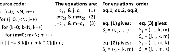
for (k=0; k<N; k++) for (m=0; m<N; m++) A[i][j] += B[k][m] + k * C[j][m];

Fo e uations’ o de

eq.1, eq.2, eq.3,

eq. (1) gives:

S1= (i, j, -, -)

eq. (2) gives:

S2= (-, -, k, m)

The equations are:

i=c₁₁ & j=c₁₂ (1) k=c₂₁& m=c₂₂ (2)

j=c₃₁ & m=c₃₂ (3) eq. (3) gives:

S₃= (i, j, k, m) S₄= (j, i, k, m) S5= (i, j, m, k)

S6= (j, i, m, k)

Figure 6: An example, eq.(3) gives different iterators nesting levels.

In general, each array is accessed (q×r) times, where q is the number of the iterations exist above its upper iterator and r is the number of the iterations exist between its upper and lower iterators. It can be easily be proved that if the unique iterators change their nesting level values without satisfying Rule 5, either the (q×r) value increases or the iterators nesting level values are given by processing another equations’ combination (it is not an issue here).

Rule 6. The nesting level values of the unique iterators are defined according to the target compiler.

According to Rule 5, the unique iterators of an equation are not inter-changed with iterators of another equation. Furthermore, in the case that they are interchanged with each other, the number of load/store and address-ing instructions will remain constant; only the number of data cache misses changes. The number of cache misses changes because multi-dimensional arrays, access their elements from no consecutive main memory locations, e.g. if i and j iterators in Fig. 6 are interchanged, A is no further accessed row-wise but column-wise from main memory; however, the data array layout is found next. Apart from reducing the number of data cache misses, there is no use to interchange these iterators. Thus, only these nesting level values accessing the array row-wise are taken for now (C compiler stores the arrays row-wise in main memory), decreasing the number of the data cache misses, e.g. for A(i, j), the i iterator is defined as the outermost one.

3.6. Decrease the number of L1 data cache accesses and the exploration space - utilizing the Register File (RF) size

exploration space. For each iteration space has been created so far, loop tiling for the RF is applied. To utilize the RF size, RF inequalities are produced giving all the (near)-optimum tile sizes. These inequalities contain i) the number of the registers needed for each array reference and for scalar variables, ii) the shape of each array’s tile.

The register file inequality is given by:

0.8×RF s≤Liter+V ar+ws+R1 +R2+...+R_n≤1.2×RF s (1)

whereRF sis the number of the available registers, L iter is the number of the different iterator references exist in the loop body, V ar is the number of scalar variables,ws is the number of the working space registers, i.e. vari-ables for intermediate results andRi is the number of the variables/registers

allocated for the i-th array.

Ri is given by: Ri =it′1×it2′ ×...×it′n, where the integerit′i are the unroll

factor values of the iterators exist in the array’s subscript, e.g. for B(i, j) and C(i, i), RB = i′ ×j′ (rectangular tile) and RC = i′ (diagonal line tile)

respectively, where i′ _{and j}′ _{are the unroll factors ofi, j iterators.}

Rule 7. Each subscript equation contributes to the creation of ineq.( 1), i.e. equation i gives Ri and specifies its expression.

The iterators are tiled and the new tiled iterators are fully unrolled, according to the RF size, to exploit data reuse; in this way, the registers are reused as many times as the number of the available registers indicate (register utilization).

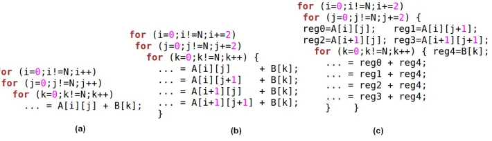
Let us give an example. In Fig. 7-a, RA = i′ ×j′ and RB = k′

vari-ables/registers are allocated for A and B arrays, respectively. If we choose a square tile for array A of size 2×2, i.e. 4 registers for A, and only 1 register for B, then the i, j iterators are tiled and the new tiled iterators are fully unrolled (Fig. 7-b). Then, by assigning the array references into registers, data reuse is achieved (Fig. 7-c). In Fig. 7-a, the (A,B) arrays are accessed (1, N2

) times while in Fig. 7-c (1, N2

/4) times, respectively.

5. . Α ιο οίη η ο α χ ίο α αχω η ώ

 Δη ιο ο αι α ι ώ ι οι ο οί ι χο

ο α ιθ ό α αχω η ώ ο α αι ί αι ια άθ ί α α αι άθ αβ η ή ο χή α άθ

 Η α ί ω η ο α χ ίο α αχω η ώ ί αι α ό

RF ≤ ≤ .

ί αι ο α ιθ ό ω α αχω η ώ άθ ί α α

Figure 7: An example, tiling for the RF is applied - we assign 4 registers for A (square tile of size 2×2) and 1 for B.

The bound values of the register file inequality (eq.( 1)) are not tight because the output code is C-code and during its compilation (translate the C-code into binary code), the compiler may not allocate the exact number of desirable addressing variables into registers. However, if assembly code would be produced instead of C-code, the register utilization would be the optimum.

The number ofL iterand wsregisters is found after the allocation of the array elements into variables/registers, because they depend on the number of tiled iterators. The ws value depends on the target compiler and this is why it is found approximately; the bounds of the RF inequality are not tight for this reason too. The goal is to store all the inner loop reused array elements and scalar variables into registers minimizing the number of register spills.

Statement 10. All schedules satisfying ineq.( 1), decrease the number of L1 data cache accesses.

Statement 11. All schedules with different number of assigned variables/registers than these the proposed methodology gives, are not considered, decreasing the exploration space.

Rule 9. Each different set of it′

i values satisfying ineq.( 1), gives a different schedule. All different it′

i values satisfying ineq.( 1) are examined.

Rule 10. TheRi values of ineq.(1), are given by Rules 11- 18 .

Rule 11. The innermost iterator is never tiled because data reuse is de-creased; if iti is the innermost iterator, then it′i = 1.

Proof 4. By tiling the innermost iterator, e.g. iterator k in Fig. 7, the array references-equations which contain it, will change their values in each iteration; this means that i) a different element is accessed in each k iteration and thus a huge number of different registers is needed for these arrays, ii) all these registers are not reused (a different element is accessed in each iteration). Thus, by tiling the innermost iterator, more registers are needed which do not achieve data reuse; this leads to low RF utilization.

Rule 12. The type1 array references which contain all the loop kernel iter-ators, do not achieve data reuse; thus only one register is needed for these arrays, i.e. Ri = 1

Proof 5. The subscript equations of these arrays change their values in each iteration vector and thus a different element is fetched in each iteration.

Rule 13. If the proposed transformation (Statement 3) is applied to eq.(i), then only one register is needed for this array reference, i.e. Ri = 1.

Proof 6. In this case, the optimum data reuse for this array is achieved since each array’s element is fetched just once (all array elements are fetched in-order); thus only one register is needed for this array, e.g. in Fig. 4, A[c]

needs only one register.

Rule 14. If the proposed transformation (Statement 3) is applied to eq.(i), then the eq.(i) iterators are never tiled and thus it′

i = 1. Otherwise, the

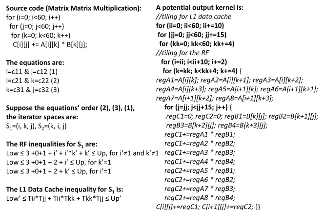
Source code (Matrix Matrix Multiplication):

for (i=0; i<60; i++) for (j=0; j<60; j++)

for (k=0; k<60; k++) C[i][j] += A[i][k] * B[k][j];

The equations are:

i=c11 & j=c12 (1) i=c21 & k=c22 (2) k=c31 & j=c32 (3)

Suppose the e uations’ o de , , ,

the iterator spaces are:

S1=(i, k, j), S2=(k, i, j)

The RF inequalities for S₁are:

Low ≤ +0+ + i’ + i’*k’ + k’ ≤ Up, for i’≠ and k’≠ Low ≤ +0+ + + i’ ≤ Up, for k’=

Low ≤ +0+ + + k’ ≤ Up, for i’=

The L1 Data Cache inequality for S₁is: Low’ ≤ Tii*Tjj + Tii*Tkk + Tkk*Tjj≤ Up’

A potential output kernel is: //tiling for L1 data cache for (ii=0; ii<60; ii+=10)

for (jj=0; jj<60; jj+=15) for (kk=0; kk<60; kk+=4) //tiling for the RF

for (i=ii; i<ii+10; i+=2) for (k=kk; k<kk+4; k+=4) {

regA1=A[i][k]; regA2=A[i][k+1]; regA3=A[i][k+2]; regA4=A[i][k+3]; regA5=A[i+1][k]; regA6=A[i+1][k+1]; regA7=A[i+1][k+2]; regA8=A[i+1][k+3];

for (j=jj; j<jj+15; j++){

regC1=0; regC2=0; regB1=B[k][j]; regB2=B[k+1][j]; regB3=B[k+2][j]; regB4=B[k+3][j];

regC1+=regA1 * regB1; regC1+=regA2 * regB2; regC1+=regA3 * regB3; regC1+=regA4 * regB4; regC2+=regA5 * regB1; regC2+=regA6 * regB2; regC2+=regA7 * regB3; regC2+=regA8 * regB4; C[i][j]+=regC1; C[i+1][j]+=regC2;}}

Figure 8: An example, Matrix Matrix Multiplication (MMM) algorithm.

Let us give an example, Fig. 3. If the proposed transformation is applied to eq.(1), then the B array’s iterators cannot be tiled and thus only one variable/register is needed for B array.

Rule 15. If there is a type1 array reference i) containing more than one iterators and one of them is the innermost one and ii) all ineq.( 1) iterators which do not exist in this array reference have unroll factor values equal to 1, then only one register is needed for this array, i.e. Ri = 1. This gives more than one register file inequalities.

Proof 7. When Rule 15 holds, a different array’s element is fetched in each iteration vector, as the subscript equation changes its value in each iteration. Thus, no data reuse is achieved and only one register is used. On the contrary, in the case that at least one iterator which do not exist in this array reference is tiled, common array references occur inside the loop body (e.g. regC1 is reused 3 times in Fig. 8); data reuse is achieved in this case and thus another RF inequality is created.

needed for this array; however, according to Rule 15, C array needs i′ _×1 registers if k′ _{6= 1 and 1 register otherwise (ifk}′ _{= 1 then the C array fetches} a different element in each iteration vector and thus only one register is needed). The array A needs i′_×k′ _{registers while B array needs k}′ _registers if i′ _{6= 1 and 1 register otherwise. Note that if the i-loop is not tiled (i}′ _{= 0),} the B and C array elements are not reused and there is 1 register for C and 1 register for B (Rule 15). The innermost iterator (j) is not tiled according to the Rule 11 (data reuse is decreased in this case).

Rule 16. We can decrease the number of it′

i values satisfying ineq.(1), by utilizing the L1 data cache line size. Regarding 1-d arrays, we can select the

it′

i values to be either 1 or multiples of the L1 cache line size. Regarding

multidimensional arrays, we can select the it′

i values which correspond to the x-axis, to be either 1 or multiples of the L1 cache line size. The arrays must be written into main memory aligned.

Moreover, there are cases that data reuse utilization is more complicated as common array elements may be accessed not in each iteration, but in each k iterations, where k ≥ 1. This holds only for type2 equations (e.g. ai+bj+c) where k = b/a is an integer (data reuse is achieved in each k iterations). The proposed methodology exploits data reuse only when k = 1 here (Rule 17) as for larger k values, the data reuse is low. For example, at Gaussian Blur algorithm (Subsection 3.10), each time the filter is shifted by one position to the right (mc iterator), 20 elements of in array are reused (reuse between consecutive iterations here, i.e. k = 1).

Rule 17. Arrays with type2 subscript equations which have equal coefficient absolute values (e.g. ai+bj+c, where a== ±b) fetch identical elements in consecutive iterations; data reuse is exploited by interchanging the registers values in each iteration. An extra RF inequality is produced for this case.

Proof 8. The above arrays access their elements in patterns. As the inner-most iterator (let j) changes its value, the elements are accessed in a pattern, i.e. A[p], A[p+b], A[p+ 2×b]etc. When the outermost iterator changes its value, this pattern is repeated, shifted by one position to the right (A[p+b],

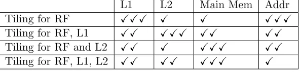
Table 1: How tiling affects the number of memories accesses and addressing instructions; the more the ticks are, the less the number of accesses / addressing instructions, are.

L1 L2 Main Mem Addr

Tiling for RF XXX X X XXX

Tiling for RF, L1 XX XXX XX XX

Tiling for RF and L2 XX X XXX XX

Tiling for RF, L1, L2 XX XX XXX X

To exploit data reuse of Rule 17, all the array’s registers interchange their values in each iteration, e.g. in (Fig. 10 - a1.2), the (in0, in1, in2, in3, in4, in5) variables interchanging their values in each iteration.

Rule 18. Regarding very small arrays (e.g. filters in image processing al-gorithms), it is tested whether their iterators are fully unrolled or not (both solutions are taken).

To sum up, by applying loop tiling for the RF, as explained above, the numbers of i) load/store instructions (or equivalent the number of L1 data cache accesses) and ii) addressing instructions, are decreased. The number of addressing instructions is decreased for three reasons. Firstly, the array references are replaced by scalar variables and thus the address computations are simplified, e.g. A(i, j) is replaced by reg variable. Secondly, several common subscript expressions which occur by unrolling the loops are replaced by scalar variables, e.g. the array references array(i+j), array(i +j + 1), array(i +j + 2) and array(i +j + 3) are replaced by array(temp), array(temp+1),array(temp+2) andarray(temp+3) respectively. Thirdly, loop unroll always decreases the number of addressing instructions.

3.7. Decrease the number of data cache and main memory accesses and the exploration space - utilizing the Data Cache memories parameters

The data cache memories sizes and the subscript equations are fully exploited, decreasing the number of data cache / main memory accesses and the exploration space. To utilize the data cache sizes, a data cache inequality for each data cache is produced, giving all the (near)-optimum tile sizes. Each inequality contains i) the tile size of each array and ii) the shape of each array tile.

of data cache architecture, 1 level of tiling (either for L1 or L2 data cache), 2 levels of tiling and no tiling solutions, are applied to all the solutions-schedules that have been produced so far. The optimum number of levels of tiling cannot easily be found since the data locality advantage may be lost by the required insertion of extra load/store and addressing instructions, which degrade performance (Table 1). In table 1, we can see how tiling affects the number of data cache accesses and addressing instructions, e.g. if the performance critical parameter is the number of L1 data cache accesses or the number of addressing instructions, then tiling is not applied for data cache. The separate memories optimization gives a different schedule for each memory and these schedules cannot coexist, as by refining one, degrading another; thus, either a sub-optimum schedule for all the memories or a (near)-optimum schedule only for one memory can be produced. However, if the goal is the minimum number of data accesses for a specific memory (let Li),

loop tiling only for Li−1 is applied.

For the reminder of this paper, we refer to architectures having separate L1 data and instruction cache (vast majority of architectures). In this case, the program code always fits in L1 instruction cache since we optimize loop kernels only, whose code size is small; thus, upper level unified/shared caches, if exist, contain only data. On the other hand, if a unified L1 cache exists, memory management becomes very complicated.

Loop tiling is applied to category-1 and category-2a arrays only (Sub-sect. 3.1). The tiles of Category-1 arrays achieve data reuse and therefore they must definitely fit in data cache. Although category-2a tiles are not reused, they have to fit in data cache to avoid cache conflicts with the category-1 ones; in this way Category-1 tiles remain in data cache. Further-more, Category-2b arrays cannot be partitioned into tiles as their elements are accessed in a ’random’ way; this leads to a large number of data cache conflicts due to the cache modulo effect (especially for large arrays). To eliminate these conflicts, Rule 19 is introduced.

Rule 19. For all the Category-2b arrays, data cache size which equals to the size of one cache way is granted. In other words, an empty cache line is granted for each different modulo (with respect to the size of the cache) of these arrays memory addresses.

Rule 20. For each register file inequality solution (schedule) produced so far, loop tiling is applied for all data cache memories and for all valid data cache tile sizes (ineq.( 2)). All tile sizes do not satisfy ineq.( 2), are not considered, decreasing the exploration space.

The data cache inequality is given by:

0.6×Lk×

(assoc−v)

assoc ≤T ile1+...+T ilen ≤1.1×Lk×

(assoc−v) assoc (2) where Lk is the k-level data cache size, assoc is the data cache

associa-tivity (for an 8-way associative data cache, assoc= 8). v value is zero when no Category-2b array exist and one if at least one Category-2b array exists. T ilei is the tile size of the ith array andT ilei =T1′×T2′×T_n′×ElementSize, where T′

i is the unroll factor of the i iterator and ElementSizeis the size of

each array’s element in bytes (T ilei refers only to 1 and

Category-2a, array). The tiling inequality of Matrix-Matrix Multiplication algorithm is shown in Fig. 8, e.g. T ileC =Tii×Tjj where Tii= 10 and Tjj = 15.

Regarding data cache tile sizes, they have to be multiples of the RF tiles sizes. Also, the tile sizes produced by L2 data cache, must be multiples of the tiles sizes produced by L1 data cache and RF (otherwise, a large number of addressing instructions is needed). Thus, the exploration space is further decreased.

The inequality bound values are not tight, i.e. 0.6 and 1.1, because smaller/larger tile sizes which divide exactly the array sizes, may achieve a lower number of addressing instructions (e.g. having an array of 2048 elements and only 800 fit in data cache, a tile size of 512 will achieve a lower number of addressing instructions than this of 800).

Statement 12. Each different set of T′

i values satisfying ineq.( 2) gives a different schedule

Statement 13. All schedules satisfying ineq.( 2) decrease the number of data cache / main memory accesses.

Proof 9. Likewise Statement 10.

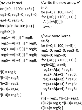
//MVM kernel for (i=0; i! 100; i+=5) { reg1=0; reg2=0; reg3=0; reg4=0; reg5=0;

for (j=0; j!=100; j++) { regB=X[j];

reg1+=A[i][j] * regB; reg2+=A[i+1][j] * regB; reg3+=A[i+2][j] * regB; reg4+=A[i+3][j] * regB; reg5+=A[i+4][j] * regB; }

Y[i] = reg1; Y[i+1]= reg2; Y[i+2]= reg3; Y[i+3]= reg4; Y[i+4]= reg5; }

//write the new array, A’

a=0;

for (i=0; i! 100; i+=5) for (j=0; j!=100; j++) {

A’[a]=A[i][j]; a++;}

//new MVM kernel a=-5;

for (i=0; i! 100; i+=5) { reg1=0; reg2=0; reg3=0; reg4=0; reg5=0;

for (j=0; j!=100; j++) { regB=X[j]; a+=5;

reg1+=A[a] * regB; reg2+=A[a+1] * regB; reg3+=A[a+2] * regB; reg4+=A[a+3] * regB; reg5+=A[a+4] * regB; }

Y[i] = reg1; Y[i+1]= reg2; Y[i+2]= reg3; Y[i+3]= reg4; Y[i+4]= reg5; }

Figure 9: Two potential output schedules for Matrix Vector Multiplication (MVM) algorithm. The code shown at the right is produced by changing the data array layout of that shown at the left.

Statement 14. The nesting level values of the new tiling iterators are found theoretically (no exploration is applied)

The nesting level values of the new (tiling) iterators are computed. For each different schedule produced by ineq.( 2), The proposed methodology computes the total number of data accesses for all the different nesting level values and the best are selected.

The number of each array’s accesses is found by:

DataAccesses=n×T ile size in elements×N um of tiles, where n is the number of times each tile is fetched and equals to (q×r), whereq is the number of iterations exist above the upper iterator of the array’s equation and r is the number of iterations exist between the upper and the lower iterators of the array’s equation.

3.8. Find the optimum data array layouts and decrease the exploration space

At this step, the (near)-optimum data array layouts are found. In this way, the spatial data reuse is further utilized and the number of data cache misses is further decreased. For each schedule produced so far, the data array layouts change; both the schedules with the new data array layouts and not, are propagated to the next step. Both solutions are taken as by changing the data array layout the additional cost of re-writing the array to main memory may be high and the number of addressing instructions is increased. However, there are several cases that by changing the data array layout, the performance is increased, i.e. a) if the array whose layout is changed is reused several times, e.g. MMM, b) if the data array layout is precomputed, c) if the input data are produced by the current application at run time; in this case, the initialization and the change of the layout, are made together, decreasing the overhead.

By changing the data array layout, the tiles are written in consecutive main memory locations, i.e. just as they are fetched (tile-wise) according to the new schedule, to increase main memory page and data cache line utilization. In this way the number of the data cache misses is highly decreased. The multi-dimensional arrays are transformed into 1-d arrays having tile-wise data layout in main memory, e.g. Fig. 9. To change the data array layouts, the array subscripts are changed-simplified, i.e. for each array reference a new variable is replacing the previous subscript equation and extra addressing instructions are inserted; these addressing instructions increase/decrease the subscripts values.

Rule 21. If the number of the arrays is larger than the data cache associativ-ity value, all the array tiles are stored into one array interleaved and tile-wise to eliminate the number of data cache misses due to the cache modulo effect. To do this, all the arrays are partitioned into identical number of tiles.

In general, compilers and related works apply loop tiling without taking into account the data array layouts. In the case that the arrays are not written tile-wise in main memory, tiling cannot give a small number of data cache misses for multi-dimensional arrays because tiles are comprised by array sub-rows which are written in different main memory locations; this means that the sub-rows will conflict with each other and thus the tiles do not remain in data cache.

3.9. Create final code and enumerate all solutions

At this step, all the solutions-schedules that have been produced so far, are transformed into C-code. These codes are compiled by the target architecture compiler and the binaries run to the target platform to find the fastest one. Each binary is run only once. Given the input size and the input data type (e.g. float, double), we do not use different input sets, as the proposed methodology optimizes applications which are not affected by the data values (see second paragraph of Section 3). It is important to say that if the input size or the input data type changes, the whole procedure is repeated, as the (near)-optimum schedule normally changes.

The number of the binaries tested depends on the application and on the hardware parameters; the number of binaries tested are from 1000 up to 100000 (the application execution time affects the compilation time). However, we can find a solution very close to the best very fast, by testing an orders of magnitude lower number of binaries. This is achieved by selecting only a few sets of different tile sizes for the data caches; performance is not highly affected by changing the data cache tile sizes, suffice they satisfy the proposed inequalities, i.e. tiles fit in the cache.

In the case that the schedule with the minimum number of data accesses for a specific memory is needed, the compilation time is very small as i) the procedure explained in Subsect. 3.7 is applied only for this memory (1 level of tiling) and ii) given that only the minimum number of data accesses is needed (the number of instructions is not taken into account here), it is possible to estimate their number, for each schedule, instead of running the schedules on the target platform.

3.10. Motivation Example (Gaussian Blur)

Table 2: Iteration spaces for the Gaussian Blur C-code.

iteration spaces Different

combinations Iteration spaces (common spaces occur)

eq.(4)-eq.(5)-eq.(6) S1 = (r, c, mr, mc),S2 = (c, r, mr, mc)

eq.(4)-eq.(6)-eq.(5) S1,S2,S3= (r, c, mc, mr),S4 = (c, r, mc, mr)

eq.(5)-eq.(4)-eq.(6) S5 = (r, mr, c, mc),S6 = (r, mr, mc, c) S7 = (mr, r, c, mc),S8 = (mr, r, mc, c) S9 = (c21, k1, c22, k2)

eq.(5)-eq.(6)-eq.(4) S5,S6,S7,S8,S9

eq.(6)-eq.(4)-eq.(5) S10= (mr, mc, r, c),S11= (mr, mc, c, r) S12= (mc, mr, r, c),S13= (mc, mr, c, r)

eq.(6)-eq.(5)-eq.(4) S10,S11,S12,S13

Iteration spaces which are excluded P1 = (r, mc, c, mr),P2 = (r, mc, mr, c) P3 = (mc, r, c, mr),P4 = (mc, r, mr, c) P5 = (c, mr, r, mc),P6 = (c, mr, mc, r) P7 = (mr, c, r, mc),P8 = (mr, c, mc, r) P9 = (c, mc, r, mr),P10= (c, mc, mr, r) P11= (mc, c, r, mr),P12= (mc, c, mr, r)

P13= (c22, k2, c21, k1)

c11, c =c12) (eq.(1)), (r+mr−2 =c21, c+mc−2 =c22) (eq.(2)), (mr= c31, mc=c32) (eq.(3)).

The proposed methodology processes the subscript equations one by one, for six different combinations, to create all the iteration spaces (Subsec-tion 3.4 and Subsec(Subsec-tion 3.5). The itera(Subsec-tion spaces created, are shown in Table 2 (S1−S13). Table 2 also shows the iteration spaces which are excluded (P1−P13), decreasing the exploration space. The number of iteration spaces is further increased (Statement 8).

For each one of the S1 − S13 iteration spaces, the register file size is utilized. Regarding S1, four register file inequalities are produced. The first of the four is the following:

0.8×RF s≤3 + 2 + 2 +r′_×c′_{+ 1 +mr}′ _{≤1.2×RF s, ifc6= 1 orr 6= 1} A potential solution (r′ _{= 2,c}′ _{= 2,mr}′ _{= 1) of the above RF inequality} is shown at the left of Fig. 10. Rin = 1 (only one register is used for this

values of the RF inequality correspond to the Liter, V ar and wsrespectively

(they are found after the register assignment); Liter = 3 becausemr, mcand

c iterators exist in the innermost loop, V ar = 2 because addr1 and addr2 variables exist andws = 2; the size of thewsdepends on the target compiler and it is found approximately. The second inequality is given due to the Rule 15 and is the following:

0.8×RF s≤4 + 0 + 2 + 1 + 1 + 1≤1.2×RF s, if c= 1 andr= 1 Rmask = 1 because of the Rule 15.

Furthermore, if Rule 17 is applied the data reuse between different itera-tions (registers in0−in5) is exploited too, giving the following inequality (a potential solution of this inequality is shown at the right of Fig. 10).

0.8×RF s≤3 + 1 + 2 +r′_×c′_+r′_×mr′_×c′_+mr′ _{≤1.2×RF s, if c}′ _≻1 The fourth inequality is produced if the mask array iterators are fully unrolled and all the array references are replaced by their constant values (Rule 18 - the mask array does not further exist). In this case the iteration space is reduced to S1 = (r, c) and R_out = 1, R_in = 1.

To sum up, all the different values satisfying the above inequalities are possible solutions. This is repeated for all the iteration spaces, i.e. S1−S13. All the schedules produced so far are further tiled according to the L1 data cache size, Subsect. 3.4 (solutions that utilize both the register file and the data cache and solution that utilize only the register file).

The L1 inequality is:

0.6×L1≤Tr×Tc+ (Tr+mr)×(Tc+mc) +Tmr×Tmc≤1.1×L1

All the tile sizes are multiples of the corresponding register file tile sizes. The nesting level values of the tiling iterators are computed as explained in Subsect.3.4.

A1.1)

for (row = 2; row < N-2; row+=2) { for (col = 2; col < M-2; col+=2) {

out0=0;out1=0;out2=0;out3=0;

for (mr=0; mr<5; mr++) {addr1=row+mr-2;

for (mc=0; mc<5; mc++) {

addr2=col+mc-2; reg_mask=mask[mr][mc];

out0+= (in[addr1][addr2] * reg_mask) / 159; out1+= (in[addr1][addr2+1] * reg_mask) / 159; out2+= (in[addr1+1][addr2] * reg_mask) / 159; out3+= (in[addr1+1][addr2+1] * reg_mask) / 159;

} } out[row][col]=out0; out[row][col+1]=out1; out[row+1][col]=out2; out[row+1][col+1]=out3; }}

A1.2)

for (row = 2; row < N-2; row++) { for (col = 2; col < M-2; col+=6) {

out0=0;out1=0;out2=0;out3=0;out4=0;out5=0; for (mr=0; mr<5; mr++) {

addr1=row+mr-2; in0=in[addr1][col-2]; in1=in[addr1][col-1]; in2=in[addr1][col]; in3=in[addr1][col+1]; in4=in[addr1][col+2];

for (mc=0; mc<5; mc++) { reg_mask=mask[mr][mc];

in5=in[addr1][col+3+mc]; out0+= (in0 * reg_mask) / 159; out1+= (in1 * reg_mask) / 159; out2 += (in2 * reg_mask) / 159; out3+= (in3 * reg_mask) / 159; out4+= (in4 * reg_mask) / 159; out5+= (in5 * reg_mask) / 159; in0=in1; in1=in2; in2=in3; in3=in4; in4=in5;

} }

out[row][col]=out0; out[row][col+1]=out1; out[row][col+2]=out2; out[row][col+3]=out3; out[row][col+4]=out4; out[row][col+5]=out5;

} }

// FIR

// BTMVM // MVM // MMM

(a)

(b)

(c)

(d)

(e)

(f)

(g) // Gaussian Blur

// BTMVM on Simplescalar

(f)

// FIR on Intel

(g)

4. Experimental Results

4.1. Experimental Setup

The experimental results presented in this section, were carried out on i) a desktop PC with Intel i7 3930K at 3.2 GHz, ii) a Virtex-5 FPGA ML507 Evaluation Platform (SDK 12.4) using PowerPC-440 processor and iii) SimpleScalar simulator [1]. The proposed methodology is compared with i) gcc and clang compilers, ii) iterative compilation technique. In (i), the operating system Ubuntu 14.04 LTS is used and two different compilers, i.e. gcc 4.6.3 and clang 3.0. In (ii), only gcc compiler is used. In (iii), the sslittle-na-sstrix-gcc compiler is used which supports out of order execution. Optimization level -O3 was used at all cases. The proposed methodology is not compared with the SOA libraries such as ATLAS or OpenCV, because they use the SIMD instructions and thus a comparison would be unfair (these libraries are also algorithm specific and the final code is not produced automatically).

The comparison is done for 5 well-known data dominant kernels of lin-ear algebra, image processing and signal processing. These are: Matrix-Matrix Multiplication (MMM), Matrix-Matrix-Vector Multiplication (MVM), Gaus-sian Blur (5 ×5 filter), Finite Impulse Response filter (FIR) and Bisym-metric Toeplitz Matrix-Vector Multiplication (BTMVM). The C-codes of these algorithms are shown in Fig. 11-(a)-(e). These algorithms are mainly selected because they are well known and simple; thus, the reader can easily understand the results (e.g. how tiling for data cache is applied), which are explained in detail.

4.2. Performance Comparison

3.9 4.2 4.6

5.3

6.8

8.1

7.5 8.4

9.1

11.7

14.4

18.3

1.8 2.0 2.2 2.4 2.9

3.3

0.0 2.0 4.0 6.0 8.0 10.0 12.0 14.0 16.0 18.0 20.0

128 256 512 1024 2048 4096

S

p

e

e

d

u

p

Rectagular Matrices of Size N

MMM

gcc on Intel i7 3930K

clang on Intel i7 3930K

gcc on PowerPC 440

Figure 12: Performance comparison of the proposed methodology and gcc/clang compilers

for MMM. The size refer toN of Fig. 11-a.

given by (Unoptimized code in gcc) / (optimized code in gcc), while the speedup for clang by (Unoptimized code in clang) / (optimized code in clang). The proposed methodology achieves higher speedup values on Intel than on PowerPC; PowerPC compiler is more aggressive (it applies more efficient transformations to the benchmark codes), resulting to faster binary code. The speedup values are from 1.8 up to 18 and from 1.9 up to 4.2, for Intel and PowerPC, respectively. As it was expected, at all algorithms, the speedup increases according to the input size; as the memory size increases, the memory management problem becomes more critical. Regarding MMM and Gaussian Blur, the proposed methodology achieves the largest speedup values (Fig. 12, Fig. 13), as i) their arrays are of larger size and ii) these algorithms have more data reuse; memory management has a larger effect in such cases. A more detailed analysis for each algorithm, follows.

1.7 1.9

2.3 2.3 2.5

2.7

2.2 2.4

2.7 2.8

3.0

3.3

1.7 1.8 1.9

2.0 2.2 2.3 0.0 0.5 1.0 1.5 2.0 2.5 3.0 3.5

512 1024 2048 4096 8196 16384

S p e e d u p

Rectagular Matrix of size M

MVM

gcc on Intel i7 3930K

clang on Intel i7 3930K

gcc on PowerPC 440

Figure 13: Performance comparison of the proposed methodology and gcc/clang compilers

for MVM. The size refer to M of Fig. 11-b.

1.9 2.1 2.2

2.4 2.5 2.6

1.8 1.9 2.0 2.0 2.1

2.2 3.5 3.8 4.0 4.2 4.4 4.7 0.0 0.5 1.0 1.5 2.0 2.5 3.0 3.5 4.0 4.5 5.0

512 1024 2048 4096 8196 16384

S p e e d u p

Matrix Size N

BTMVM

gcc on Intel i7 3930K

clang on Intel i7 3930K

gcc on PowerPC 440

Figure 14: Performance comparison of the proposed methodology and gcc/clang compilers

1.8 1.8 1.9 2.1 2.3 2.4 2.1 2.2 2.4 2.5 2.7 2.8 1.8 1.9 2.0 2.1 2.2 2.3 0.0 0.5 1.0 1.5 2.0 2.5 3.0

(200,20) (400,40) (640,60) (1000,100) (2000,200) (4000,500)

S p e e d u p

Matrix Sizes (n, ksize)

FIR

gcc on Intel i7 3930K

clang on Intel i7 3930K

gcc on PowerPC 440

Figure 15: Performance comparison of the proposed methodology and gcc/clang compilers for FIR. The sizes refer to (n, ksize) of Fig. 11-c.

2.5 2.6 2.8 2.9 3.2 3.5 2.6 2.7 2.9 2.9 3.3 3.6 2.2 2.3 2.6 2.8 3.1 3.4 0 0.5 1 1.5 2 2.5 3 3.5 4

128x128 256x256 512x512 800x600 1024x1024 2048x2048

S p e e d u p

Matrix Sizes (N x M)

Gaussian Blur

gcc on Intel i7 3930K

clang on Intel i7 3930K

gcc on PowerPC 440

and thus a smaller speedup is achieved (from 1.8 up to 3.3). Regarding the proposed methodology output C-codes, gcc produces about 1.5 times faster binaries. Gcc, clang and all other related tools and libraries, apply loop tiling without taking into account the data array layouts and the memory hierarchy parameters; this leads to a large number of data cache misses (it is explained in the last paragraph of Subsect. 3.8). In the case that L2 ≻ (4×N2

) (B array fits in L2), the best schedule found applies loop tiling only for L1 data cache as follows. The arrays are partitioned in such a way that two rows of A and p1 columns of B fit in L1 (the proposed methodology gives column-wise layout for B); when the first row of A is multiplied by p1 columns of B, the next row of A is fetched and it is multiplied by the same columns of B as before etc. For larger array sizes, there is no p1 number that two rows of A and p1 columns of B fit in L1 and this is why the arrays have to be partitioned even more; in this case, the proposed methodology applies loop tiling for L2 cache too, i.e. 3 rectangular tiles (one for each matrix) have to fit in L2. It is important to say that in this case, sub-rows of A are multiplied by sub-columns of B; however, the sub-rows elements are not written in consecutive main memory locations and this is why the number of data cache misses is highly increased. Thus, when the MMM arrays are partitioned into rectangular tiles, their data layouts must change (A and B arrays), from row-wise to tile-wise (the change of the layouts is included to the execution time).

Regarding MVM (Fig. 13), gcc produces higher quality code than clang. The best schedules produced by the proposed methodology use k registers for Y, 1 for A and 1 for X. The output schedules are similar to that shown in Fig. 13. Changing the data array layout of matrix A is not performance efficient here because i) A array is very large compared to the others (Y,X), ii) it is not reused (each element of A is accessed only once). Regarding Intel processor, tiling for data cache is not performance efficient here since the reused arrays, i.e. Y and X, are small and they fit in data cache in most cases. On the other hand, tiling for data cache is applied for PowerPC processor (large array sizes only). The best tiling solutions for MVM that the proposed methodology gives are as follows. The matrix A is partitioned in rectangular tiles of size r×c where c≫r and the array X is partitioned into tiles of size c; the schedule defines that each tile of X is multiplied by all possible tiles of A.

the performance of PowerPC processor sinceabs() routine needs more cycles at PowerPC than at Intel. Also, clang produces slightly faster binaries than gcc for the benchmark code here. The C-code produced by the proposed methodology here is similar to that shown at the right of Fig. 11-(f) (more registers for Y and A are used). The proposed methodology assigns A array elements into registers which interchange their values in each iteration (Rule 17 has been applied); thus a smaller number of abs functions is executed increasing performance even more. Loop tiling for L1 is applied only for PowerPC as the array sizes are small in contrast to the large Pentium cache sizes.

Regarding FIR (Fig. 15), the proposed methodology achieves the lowest performance gain, as FIR arrays have very small size and data reuse is small. The proposed methodology output code for clang compiler is shown at the left of Fig. 11-(g) (double precision floating point values). For double precision floating point values, clang and gcc use the XMM registers of Pentium and this is why 15 variables are used for the FIR arrays (Intel contains 16 XMM registers). Loop tiling for L1 is applied only for PowerPC as the array sizes are small in contrast to the large Pentium caches.

Regarding Gaussian Blur (Fig. 16), the speedups are about the same at all cases. The schedules shown in Fig. 10 achieve high execution speed at both processors. The schedules with tile-wise layout for input matrix, are not performance efficient because even in this case, data locality cannot be achieved. When tiling for data cache is applied, the best C-codes generated by the proposed methodology, partition the arrays vertically into parts (sub-images of size M ×p1).

4.3. Comparison on data accesses and arithmetic instructions