Internship Report on benchmarking of Python based turbine model of cost of energy model; and generation of load coefficients to be used in the turbine model

Company

DNV-GL

Location

Groningen, The Netherlands

Duration

August 4, 2014 – November 4, 2014

Supervisors

Wouter Haans, Lindert Blonk and Menno

Kloosterman

Submitted to

Prof.Dr.ir. H.W.M. Hoeijmakers

University of Twente

The Netherlands

Submitted by

Sudip Adhikari

S1417878

M.Sc. Sustainable Energy Technology

Submitted Date

November 4,2014

PROJECT NAME

Internship Report on Benchmarking of Python

Based Turbine Model of Cost of Energy Model; and

generation of Load coefficients to be used in the

Turbine Model

Customer Name

Report No.: , Rev.

IMPORTANT NOTICE AND DISCLAIMER

1. This document is intended for the sole use of the Client as detailed on the front page of this document to whom the document is addressed and who has entered into a written agreement with the DNV GL entity issuing this document (“DNV GL”). To the extent permitted by law, neither DNV GL nor any group company (the "Group") assumes any responsibility whether in contract, tort including without limitation negligence, or otherwise howsoever, to third parties (being persons other than the Client), and no company in the Group other than DNV GL shall be liable for any loss or damage whatsoever suffered by virtue of any act, omission or default (whether arising by negligence or otherwise) by DNV GL, the Group or any of its or their servants, subcontractors or agents. This document must be read in its entirety and is subject to any assumptions and qualifications expressed therein as well as in any other relevant communications in connection with it. This document may contain detailed technical data which is intended for use only by persons possessing requisite expertise in its subject matter.

2. This document is protected by copyright and may only be reproduced and circulated in accordance with the Document Classification and associated conditions stipulated or referred to in this document and/or in DNV GL’s written agreement with the Client. No part of this document may be disclosed in any public offering memorandum, prospectus or stock exchange listing, circular or announcement without the express and prior written consent of DNV GL. A Document Classification permitting the Client to redistribute this document shall not thereby imply that DNV GL has any liability to any recipient other than the Client.

3. This document has been produced from information relating to dates and periods referred to in this document. This document does not imply that any information is not subject to change. Except and to the extent that checking or verification of information or data is expressly agreed within the written scope of its services, DNV GL shall not be responsible in any way in connection with erroneous information or data provided to it by the Client or any third party, or for the effects of any such erroneous information or data whether or not contained or referred to in this document.

4. Any wind or energy forecasts estimates or predictions are subject to factors not all of which are within the scope of the probability and uncertainties contained or referred to in this document and nothing in this document guarantees any particular wind speed or energy output.

KEY TO DOCUMENT CLASSIFICATION

Strictly Confidential : For disclosure only to named individuals within the Client’s _{organisation.}

Private and Confidential : For disclosure only to individuals directly concerned with the _{subject matter of the document within the Client’s organisation.}

Commercial in Confidence : Not to be disclosed outside the Client’s organisation.

DNV GL only : Not to be disclosed to non-DNV GL staff

Client’s Discretion :

Distribution for information only at the discretion of the Client (subject to the above Important Notice and Disclaimer and the terms of DNV GL’s written agreement with the Client).

Project name: Project Name DNV GL Energy Renewables Advisory St Vincent’s Works Silverthorne Lane Bristol BS2 0QD United Kingdom

Tel: +44 117 972 9900 GB 810 7215 67 Report title: Internship Report on Benchmarking of Python

Based Turbine Model of Cost of Energy Model; and generation of Load coefficients to be used in the Turbine Model

Customer: Customer Name

Contact person: [Contact person] Date of issue:

Project No.: [Project No.]

Report No.: , Rev.

Prepared by: Verified by: Approved by:

Sudip Adhikari

Student Placement Lindert Blonk Mechanical Engineer

Turbine Engineering

Wouter Haans

Head of Technology Evaluation Turbine Engineering

[Name]

[title] Menno Kloosterman Engineer

Turbine Engineering

[Name]

[title] [Name] [title]

☐ Strictly Confidential Keywords:

[Keywords]

☐ Private and Confidential

☒ Commercial in Confidence

☐ DNV GL only

☐ Client’s Discretion

☐ Published

Reference to part of this report which may lead to misinterpretation is not permissible.

Table of contents

1 ACKNOWLEDGEMENT ... 1

2 ABSTRACT ... 2

3 SECTION 1 - BENCHMARKING OF PYTHON BASED TURBINE MODEL OF COST OF ENERGY MODEL ... 3

3.1 Introduction 3 3.2 Objective 3 3.3 Theory – Cost of Energy 3 3.4 Methodology 5 3.5 Results 5 3.6 Conclusion 6 3.7 Recommendation 6 4 SECTION 2 - FIND BEST APPROACH TO CREATE LOAD COEFFICIENT CSV FILE ... 7

4.1 Introduction 7 4.2 Objective 7 4.3 Theory – Power Law Fit 7 4.4 Methodology 8 4.5 Results 10 4.6 Comparison of Various Load Components 17 4.7 Conclusion 22 4.8 Recommendation 22 5 REFERENCES ... 25

Appendices

APPENDIX B: PYTHON CODE FOR METHOD 1 ... 28

APPENDIX C: PYTHON CODE FOR METHOD COMPARISION... 29

List of Figures

Figure 1.1: Schematic flow diagram CoE model [2] ... 4

Figure 1.2: Low Speed Shaft Mass plot ... 5

Figure 2.1: EBR_My plot using Method 1 ... 11

Figure 2.2: EBR_My plot using Method 2 ... 11

Figure 2.3: EBR_My plot using Method 3 ... 12

Figure 2.4: EBR_My plot using Method 4 ... 12

Figure 2.5: EBR_My plot using Method 5 ... 13

Figure 2.6: EBR_My plot using Method 6 ... 13

Figure 2.7: EBR_My load plot Method 1 ... 14

Figure 2.8: EBR_My load plot Method 2 ... 15

Figure 2.9: EBR_My load plot Method 3 ... 15

Figure 2.10: EBR_My load plot Method 4... 16

Figure 2.11: EBR_My load plot Method 5... 16

Figure 2.12: EBR_My load plot Method 6... 17

Figure 2.13: EYB_Fx load plot Method 2 ... 19

Figure 2.14: FHS_MY4 load plot Method 2 ... 20

Figure 2.15: FYB_FX4 load plot Method 2 ... 20

Figure 2.16: FYB_MY4 load plot Method 2 ... 21

Figure 2.17: FHS_MY4 with correction factor ... 21

Figure 2.18: FHS_MY4 without correction factor ... 21

Figure 2.19: FYB_MY4 with correction factor ... 22

Figure 2.20: FYB_MY4 without correction factor ... 22

Figure 2.21 : Surface plot for EBR_My ... 24

List of Tables

1

ACKNOWLEDGEMENT

Internship at DNV-GL, Groningen has been a good learning opportunity for me and I had a pleasant time throughout the internship. I would like to thank Prof. Harry Hoeijmakers and Wouter Haans for providing me the opportunity to do this internship. I am thankful to Wouter Haans for his overall supervision of my work throughout the internship. Special thanks go to Lindert Blonk and Menno Kloosterman for their direct supervision of my internship. Lindert Blonk supervised for the benchmarking of Turbine model and helped me to get acquainted with Python. Menno Kloosterman supervised for generating load coefficient CSV file from the new load database, which is to be used in the Turbine model. I would also like to thank TECC - Load Database for their feedback on my work.

Finally I would like thank everyone at DNV GL – Wind group at Groningen office: Ewoud Stehouwer, Debby De Jong van Ballegooy, Lukasz Turek, Shanower Hossain and Gerrit-Jan Van Zinderen for their help and friendly environment at work.

2

ABSTRACT

This report has been prepared on the basis of internship work done during August 4, 2014 – November 4, 2014. The report has been divided into two sections, each section based on a different task assigned during the internship. Each section discusses about the

objectives, methodology, results, conclusion and recommendation for the respective task.

The first section explains the benchmarking of the python based turbine model which has been developed at DNV-GL; against the industrial data and the old excel based Turbine model. For the benchmarking task internal turbines (i.e. wind turbines designed at DNV-GL) and external turbines (i.e. wind turbines which are not designed by DNV-DNV-GL) were considered. Results of the benchmarking done against internal turbines were more useful as more turbine data were available for them. The data for the external turbines were limited. The benchmarking task was an iterative process. Results of the benchmarking were useful in identifying the bugs in the python based Turbine Model. This report only discusses about the latest benchmarking done using the internal turbines data, which was completed on October 3, 2014.

The second section describes about various methods for obtaining the power law fit coefficient for load components by using the load database available at DNV-GL. In

addition, power law fit coefficient for calculating the expected power is also obtained. The power law fit coefficients obtained are exported to a CSV file, which will be used in the Turbine Model for calculating the loads. These coefficients for various load components were obtained considering various components of load data. Scripts were written in Python to access the required data from the load database and to perform the

3

SECTION 1 - BENCHMARKING OF PYTHON BASED TURBINE

MODEL OF COST OF ENERGY MODEL

3.1

Introduction

DNV-GL is migrating from its old Excel based Cost of Energy Model for wind turbines to its new Python based Cost of Energy Model. For this purpose the Turbine Model, which is a part of the Cost of Energy Model had to be benchmarked. The benchmarking task was done by comparing the turbine component mass results obtained from the Python based Turbine Model against the results from Excel based Turbine Model and the actual data. For collecting the actual turbine data internal turbines (i.e. wind turbines designed at DNV-GL) and external turbines (i.e. wind turbines which are not designed by DNV-GL) were considered. However, more reliable data were available for internal turbines. The benchmarking task was an iterative process and was re-run after modifications were made on the basis of the benchmarking results. In this section only the latest

benchmarking done using the internal turbines data is presented.

The latest benchmarking task was done using the internal turbine data. The external turbines were not considered in the latest benchmarking as individual component masses were not available. Collective component masses (e.g. RNA mass) were only available for the external turbines. Benchmarking against collective component masses did not give a clear idea about the source of error. In a collective component mass, the error can be in positive and negative for different components and hence when they are added the final value can have a lower error; while in reality the error is high.

3.2

Objective

To perform benchmarking of the python based turbine model developed at DNV-GL.

 To compare the results obtained from the python based turbine model against the industrial turbine data available at DNV-GL database.

 To compare the results obtained from the python based turbine model against the results from the old excel based turbine model, which was also developed at DNV-GL.

3.3

Theory – Cost of Energy

CoE = _{Energy Produced}Total costs [1]

It can also be expressed as used in DNV-GL : CoE = FCR.CAPEX+OPEX_AEP [2]

Where,

CAPEX is the total capital expenditure of the farm

FCR is the fixed charge rate applied to CAPEX OPEX is the annual operating expenditures

AEP is the annual electricity production of the farm

FCR is calculated using the following relation: FCR = _1−(1+r)r _−n [2]

Where, r is the summation of inflation rate and real interest rate; and n is the number of years over which the loan runs.

Figure 1.1: Schematic flow diagram CoE model [2]

Figure 1.1 shows the schematic layout of the Cost of Energy model at DNV-GL. The model has 4 sub-models: Balance of Plant (BOP) model, Turbine model, Operation &

3.4

Methodology

Following steps were done for doing the benchmarking task:

 Twelve internal turbines were selected for the benchmarking task.

 The inputs required for running the python based turbine model and excel based turbine model were prepared. Details regarding procedure for running the python based turbine model has been attached along with this report in the attached folder. Preparation of this document was also done as part of the internship task. Steps for doing the benchmarking against internal turbines were followed from this document named

“Procedure_for_benchmarking_against_internal_and_external_turbine.docx”.

 Results from the python based turbine model and excel based turbine model along with actual turbine data were plotted in a bar graph. Python based code for this task is attached in Appendix A. Detailed code is attached in the attached folder along with this report.

3.5

Results

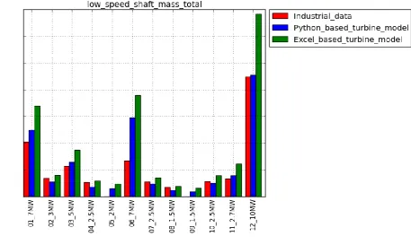
In this section the result for only one mass component is discussed. The mass value and the names of the turbines are kept confidential. Details of this plot and the other

component masses are attached in the attached folder attached along this report.

Figure 1.2 shows the low speed shaft mass plot of the actual turbine data against the results from python based turbine model and excel based turbine model. From the result we can see that the python based turbine model is showing better results for majority of turbines. However for some smaller turbines the python based turbine model is

underestimating the result. But the error is lower compared with the old excel based turbine model except for 04_2.5MW and 08_1.5MW turbines.

3.6

Conclusion

The results of benchmarking against internal turbines are more reliable and this is preferred to the benchmarking against external turbines. From the observation of the results of benchmarking against internal turbines of various mass components which has been attached in the attached folder, we find that the python based turbine model is

giving overall good results for generator frame, generator mass, hub mass, inverter mass, low speed shaft mass, nacelle cover mass, rotor blades mass, rotor pitch bearing mass, tower mass and rotor pitch system mass.

But results of main bearing housing mass, main bearing mass, yaw bearing and yaw system were not so good for some turbines. Transmission mass were high for large turbines.

3.7

Recommendation

 The mass components for which the results are not good are mentioned in

conclusion. These models need to be improved for having better results from the Python based turbine model.

 Benchmarking is an iterative process, so a set of turbines both for internal turbines and external turbines with all the necessary files to run the python based turbine model has been prepared. As a part of internship task this has been documented clearly in the document

“Procedure_for_benchmarking_against_internal_and_external_turbine.docx”. Future benchmarking can be done following this document after any change has been made to the Turbine Model.

 DNV – GL wants to have new load coefficient file, which will be based on the new load database. Once this task has been finalized it is necessary to do the

4

SECTION 2 - FIND BEST APPROACH TO CREATE LOAD

COEFFICIENT CSV FILE

4.1

Introduction

DNV-GL has been using power law fit coefficient CSV file for calculating various load components and expected power, which was created using class II turbines. This was based on the old load database. Now the company has an updated database with wide range of turbines. Based on this new load database new Power law fit coefficient were obtained. The Turbine model was run with this new Power law fit coefficient. The turbines which were used for the internal benchmarking of the turbine model were used to

evaluate the results of the new Power law fit coefficient by running the Turbine model. The actual loads with the results obtained from using the old load coefficient CSV and new load coefficient CSV were compared.

4.2

Objective

To find the best approach to calculate load and expected power coefficients using power law fit for various load components and power, to be used in the Turbine model of Cost of Energy model.

 To identify various method to do the power law fit and prepare the CSV file for each method.

 Compare the results for each method against 10 internal turbines’ loads from the load database at DNV-GL.

 Evaluate the results of various methods and suggest the best method among them with recommendation for improvement.

4.3

Theory – Power Law Fit

In load component versus diameter and power versus diameter plot, power law fit trend line gives a good fit for the data. The moments are approximately cubic with diameter and forces are approximately square with diameter. Similarly for power versus diameter, power is approximately square with diameter [3].

Power law equation is of the form:

𝑦 = 𝑘. 𝐷𝑛 _{……… (2.1)}

method can be used for fitting the data with the power law. For that we can linearize the equation (2.1) as follows:

ln 𝑦 = ln 𝑘 + 𝑛 ln 𝐷 …….. (2.2)

This equation is comparable to the linear equation 𝑦̂= mx +c ………. (2.3); where

𝑦̂= ln 𝑦

c = ln 𝑘

m =n x = ln 𝐷

The least square method gives us two equations (i.e. equation 2.4 and 2.5) which have to be solved to obtain the coefficient m and c; which will later be used to obtain the value for k and n.

∑𝑛𝑖=1𝑦𝑖 = ∑𝑛𝑖=1𝑥𝑖+ 𝑛𝑐………. (2.4)

∑𝑖=1𝑛 𝑥𝑖𝑦𝑖= 𝑚 ∑𝑛𝑖=1𝑥𝑖2+ 𝑐 ∑𝑖=1𝑛 𝑥𝑖 ………. (2.5)

For measuring the goodness of fit, Coefficient of determination also known as 𝑅2 _{is used.}

It is defined as:

𝑅2_{= 1 −}𝑆𝑆𝐸

𝑆𝑆𝑇 ……..(2.6)

Where SSE (error sum of squares) = ∑(𝑦𝑖− 𝑦̂𝑖)2

SST (total corrected sum of squares) = ∑(𝑦𝑖− 𝑦̅𝑖)2

Fit is considered perfect for 𝑅2_{= 1 and bad for 𝑅}2_{= 0}

[4]

4.4

Methodology

Following steps were followed to accomplish the objective:

 Various methods, i.e Method 1,2,3,4,5 and 6 described below were identified and used to do the power law fit to obtain the power law fit coefficient for load and expected power; which was exported to a CSV file. To run the turbine model using this CSV file, it has to be uploaded in the

“Software\Source\Engineering\CostModelling\Turbine\Loads” folder.

 Loads data were obtained for ten internal turbines. These turbines were same as the ones used in internal benchmarking.

 A comparison was done between the actual loads, loads calculated using the old CSV file and loads calculated using the new CSV file.

 Results from Method 1,2,3,4,5 and 6 were compared and one of the methods was recommended as the best approach among them.

 The above mentioned steps were done for cases using wind class correction factor and without using wind class correction factor.

The methods to obtain power law fit coefficient for load and power are described below:

Method 1: In this method Power Law fit for various load components and power is done

to give the Power Law fit coefficient. No data has been filtered.

Method 2: In this method filtering of data has been done once. Turbines which are

'Generic_10MW','NREL','seismic','SWAY' and 'Clipper' are removed in the analysis.

Method 3: Here the following steps are followed:

 From the load database, turbines which are

'Generic_10MW','NREL','seismic','SWAY' and 'Clipper' are removed. This is the first filter.

 A power law fit is done.

 Error for each turbine is calculated for each load component (e.g. EBR_Mx). Here: Error = ((Actual value of the load - Estimated value from the curve fit)/ Actual value of the load) *100

 Then a list of turbines is prepared which have more than 50% error in more than 4 load components.

 Again power law fit is done; this time excluding the list of turbines which have more than 50% error in more than 4 load components and also the turbines in first filter. This is the second filter.

 The turbines filtered in the second filter and first filter are filtered for calculating the power coefficient. The power versus diameter is also fitted using power law fit and the power law coefficients are obtained.

 Finally we obtain the new fit with new power law fit coefficients for power and load.

Method 4: Here the following steps are followed:

 From the load database, turbines which are

'Generic_10MW','NREL','seismic','SWAY' and 'Clipper' are removed. This is the first filter.

 If the turbines have same diameter with different loads, the lesser value load is multiplied by a correction factor.

 A power law fit is done.

Error = ((Actual value of the load - Estimated value from the curve fit)/ Actual value of the load) *100

 Then a list of turbines is prepared which have more than 50% error in more than 4 load components.

 Again power law fit is done; this time excluding the list of turbines which have more than 50% error in more than 4 load components and also the turbines in first filter. This is the second filter.

 Again, if the turbines have same diameter with different loads, the lesser value load is multiplied by a correction factor.

 Finally we obtain the new fit with new load power fit coefficients.

Method 5: This method follows the same steps that have been followed in the old excel

based Turbine model:

 From the load database, turbines which are

'Generic_10MW','NREL','seismic','SWAY' and 'Clipper' are removed. This is the first filter.

 Power law fit coefficients for loads and power; are obtained using the loads database.

 Using the above Power law fit coefficients; new Power law fit coefficients are calculated for different diameter.

 Finally an average Power law fit coefficients is calculated which is exported to the csv file.

 Again, a second filter is done as in method 3 and same steps are repeated to obtain the final Power law fit coefficients

Method 6: In this method fit was done for individual wind class. Turbines which are

'Generic_10MW','NREL','seismic','SWAY' and 'Clipper' are removed for this analysis. Wind class 2 power law coefficients were used later for calculating the loads.

[The python code in detail for each method is in the attached folder attached along with this report. The code for method 1 is shown in Appendix B]

4.5

Results

4.5.1

Overview of a Load Component

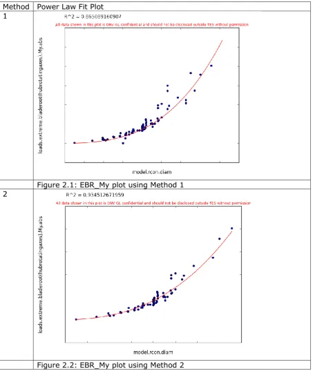
Power Law Fit Plot

load component are shown in detail in the attached folder that has been attached along with this report. Also the python code to do the power fit plot and generating the CSV file is attached. Plots shown below includes wind class correction factor for all the methods.

Method Power Law Fit Plot 1

Figure 2.1: EBR_My plot using Method 1 2

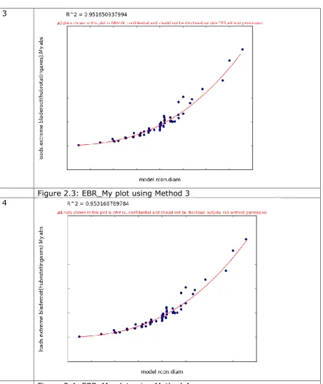
3

Figure 2.3: EBR_My plot using Method 3 4

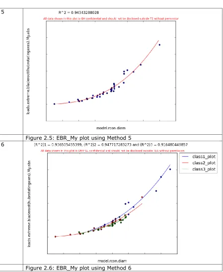
5

Figure 2.5: EBR_My plot using Method 5 6

Figure 2.6: EBR_My plot using Method 6

law fit done for individual class. This can also be a good method. But for the present analysis, turbines for individual wind class are less. In some load components we would have only 1 turbine. So method 6 is not a suitable approach for all the load components. However loads have been calculated using the CSV generated using wind class 2 data.

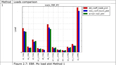
Load plot

Plots for load extreme blade root My component obtained using the new load coefficient CSV against the actual load data against the load from old load coefficient is shown in figures below. The new coefficient loads plot in the plots below means for each respective method. To protect the confidentiality of the data the scale and the names of the turbines has not been provided. Plots for this load component and other load components are shown in detail in the attached folder that has been attached along with this report. Also the python code to do the plot is attached. Plots shown below includes wind class

correction factor for all the methods. Method Loads comparison

1

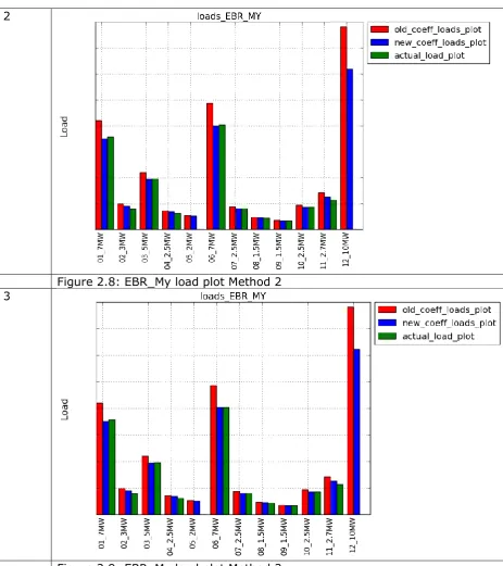
2

Figure 2.8: EBR_My load plot Method 2 3

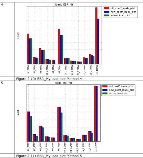
4

Figure 2.10: EBR_My load plot Method 4 5

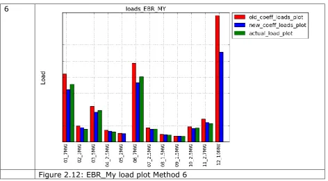
6

Figure 2.12: EBR_My load plot Method 6

Observing from Figure 2.7 to 2.12, we could see that better results were for Figure 2.8 - Method 2. The results for method 2 and 1 seem to be comparable. Figure 2.11 - Method 5 shows that instead of the results being equal to the actual load, it is equal to the result using old load coefficient. However this equality is only for this load component. Also in other load components Method 5 does not show good results.

4.6

Comparison of Various Load Components

The above results are shown for only one load component including the wind class correction factor. However to make a conclusion about the above mentioned methods both the cases using the wind class correction factor and without using the wind class correction factor should be evaluated. In addition individual methods should be compared for all the load components.

4.6.1

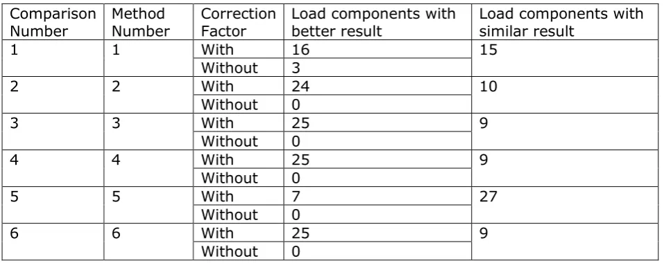
Comparison on Wind Class Correction Factor

Comparison

Number Method Number Correction Factor Load components with better result Load components with similar result

1 1 With 16 15

Without 3

2 2 With 24 10

Without 0

3 3 With 25 9

Without 0

4 4 With 25 9

Without 0

5 5 With 7 27

Without 0

6 6 With 25 9

Without 0

Table 2.1: Comparison of Methods including wind class correction factor and without including wind class correction factor

From the above Table2.1 we can see that better results were obtained for all the Methods when the wind class correction factor was included. Also there were load components where the numbers of turbines having deviation from the actual result were of same number for both the component. The detail python code used for comparing is in the attached folder that has been attached with this report. Python code for comparison is also shown in Appendix C

4.6.2

Comparison among Methods

Since including wind class correction factor had better results, only these will be included for Method comparison. Results for overall loads were evaluated for all the methods. Comparison was done between two individual methods to have a better understanding which method is better than the other. For each load component individual turbine loads were compared against the actual load. The deviation was compared between the

methods and the method with higher numbers of lesser deviation was considered a better method for that load component. The comparison method is similar to the one used in Table 2.1.

Comparison

Number Method Number Load components with better result Load components with similar result

1 1 15 5

2 14

2 2 20 7

3 7

3 1 15 5

3 14

5 2 23 1 4 10

6 2 29 2

5 3

7 2 13 8

6 13

8 2 24 6

Old_coeff 4

9 6 23 5

Old_coeff 6

Table 2.2: Comparison of various methods of power law fit

From Table 2.2 we can see that Method1 and 2 seems to be the better approach for obtaining the load coefficient CSV file to run the Turbine model. However Method 2 is chosen as it is necessary to do the first filter. Method 6 can also be considered. But in Method 6 some of the load components have only one turbine. Method 2 gives better results compared to Method 6 when we compare it with the old load coefficient.

4.6.3

Results of Method 2

Observing results from Table 2.2, Method 2 was considered the better approach;

elaboration of the results of this method is done here. Since the new load coefficient CSV is supposed to give better results than the Old load coefficient CSV, comparison between them should be done. In comparison to the load results from the Old load coefficient CSV, among 34 load components - 4 load components did not give good results. The 4 load components plots are shown below:

Figure 2.14: FHS_MY4 load plot Method 2

Figure 2.16: FYB_MY4 load plot Method 2

Observing Figure 2.13 – 2.16 we can see the new load coefficient result from Method 2 was not as good as the result from the old load coefficient for the 4 load components. But the results were comparable for smaller turbines. The deviations were higher in case of class 1 turbines. Among the four load components, two load components (i.e. EYB_FX and FYB_FX4) are not provided in the load coefficient CSV. They are calculated in the Turbine model.

Comparison of FHS_MY4 and FYB_MY4 with and without wind correction factor

Figure 2.17: FHS_MY4 with correction factor

Figure 2.19: FYB_MY4 with correction factor Figure 2.20: FYB_MY4 without correction factor

The legend for Figure2.17 – 2.20 are same as for the earlier figures (e.g. Figure 2.16). In Figure2.17 – 2.20; we can see that the load estimated from the power law fit coefficients is not comparable to the actual loads for class I turbines, the estimated loads are lower. So even after the wind class correction is done the deviation is still large.

4.7

Conclusion

Wind class correction factor which is considered in the Turbine Model gives better results for all the methods than calculating the load without the wind class correction.

Also from the analysis of the various Methods identified for different load components, Method 2 is the better approach among the six methods. But for four load components Method 2 does not seem to be a suitable approach. Among the four load components two load components are not calculated using the load coefficient CSV. So it can be said that CSV generated using Method 2 is not suitable only for two load components (i.e.

FHS_MY4 and FYB_MY4). In these load components the load is underestimated for the class 1 turbines. But the results are still comparable for smaller turbines. So overall the load coefficient CSV generated using Method 2 is suitable to be used to run the “Turbine model” among the identified six methods. Method 6 can also be considered but this method would require more turbine data to be included in the load database.

4.8

Recommendation

be done on the basis of wind class of turbines. Data should be collected for turbines and categorized on the basis of wind class. This will help to know the performance of the new load coefficient CSV in terms of wind class and also the performance of the correction factors. This might also help to find a better solution for load components FHS_MY4 and FYB_MY4 in which the results are better for the Old load coefficient CSV. In addition if the load database has more data, load coefficient CSV for individual wind class can be generated and the analysis can be done considering it too.

 Proper evaluation of the Methods for doing the power law fit can be done by giving weight to important load components. In this report all the load components are given equal weight.

 In the current turbine model, the correction factor is used while running the turbine model. The correction factor can also be added when we do the power law fit. Comparison among these two approaches can be done, to see which gives a better result.

 Changes in the turbine model have to be done so that the power law fit coefficient for load components EYB_FX and FYB_FX4 can be included in the load coefficient CSV. This will help in load calculation for these components using the coefficient obtained from the new load database instead of obtaining the values considering other load components.

 A better filtering approach should be considered. One of the approaches can be to use standard filter lists accessible from the load database GUI. Here filtering refers to the second filtering step which is done after filtering the Generic_10MW, NREL, seismic, SWAY and Clipper.

 Another method for obtaining the load coefficient would be doing the surface fit for load considering the diameter and the power density. This approach can be

5

REFERENCES

[1] J. . F. Manwell, J. G. McGowan en A. . L. Rogers , Wind Energy Explained: Theory, Design and Application, WILEY, 2009.

[2] M. Kloosterman, „Cost of Energy Model Theory Guide,” DNV - GL, 2014. [3] P. Jamieson , Innovation in Wind Turbine Design, WILEY, 2011.

APPENDIX A:

PYTHON CODE TO PLOT BENCHMARKING RESULTS

import pandas as pd

import matplotlib.pyplot as plt mport numpy as np

import os

""" The following script plots the actual industrial data available at the DNV-GL database against the result obtained from the python turbine model and the old excel cost model. If the user does not want to include theresults from the excel cost model then comment line numbers 13,14,19,28,36; and delete ",excel_data_plot[0]", ",'Excel_data'" from line 38.In order to run the script please make sure that the folder which has this script, also contains the 'batch_csv_test.csv', 'batch_results.csv' and 'excel.csv' files. In case you are not plotting the results from excelcost model,'excel.csv' is not required. """

industrial_data = pd.read_csv('batch_csv_test.csv') # batch_csv_test.csv this is the input file for the python turbine model and this file also has the industrial data of various componenets

python_data = pd.read_csv('batch_results.csv') # batch_results.csv is the result file generated by the python turbine model

excel_data = pd.read_csv('excel.csv',';') # excel.csv file is created from the excel turbine model

excel_data['yaw_system'] = excel_data['yaw_brake_Mass ']+excel_data['yaw_motor_Mass ']

pos = np.arange(len(python_data['turbine_RNA_mass']))

width = 0.27

python_data_variables =

['tower_mass_total','rotor_blades_mass_total','rotor_pitch_bearings_mass_total','rotor_pitch_systems_mass_total','hub_mas s_total','low_speed_shaft_mass_total','main_frame_mass_total','generator_frame_mass_total','main_bearings_mass_total',' main_bearing_housing_mass_total','yaw_bearing_mass_total','yaw_system_mass_total','nacelle_cover_mass_total','inverter_ mass_total','transmission_mass_total','generator_mass_total','turbine_RNA_mass']

excel_data_variables = ['Tower_Mass ','blade_set_Mass ','pitch_bearing_Mass ','pitch_system_except_bearing_Mass ','hub_Mass ','low_speed_shaft_king_pin_Mass ','bedplate_Mass ','generator_frame_Mass ','main_bearing_Mass ','main_bearing_housing_Mass ','yaw_bearing_Mass ','yaw_system','nacelle_cover_Mass ','inverter_Mass ','Drive_train_gearbox_Mass ','Drive_train_generator_Mass ','RNA_SUM_inc_drivetrain_Mass ']

count = 0 # this variable is used as index number to access the parameters in the python_data_variables and excel_data_variables and also for the plt.figure

path = 'industrial_python_excel_mass_plots' # this folder will be created in the folder which has this script; and the figure will be saved inside this folder

if not os.path.exists(path):

os.makedirs(path)

for variables in python_data_variables :

plt.figure(count)

plt.grid()

industrial_data_column = python_data_variables[count] #assigning parameter from the python_data_variables list

python_data_variables_column = python_data_variables[count]

excel_data_variables_column = excel_data_variables[count]

for check in checks:

industrial_data[industrial_data_column][check]=0

industrial_data[industrial_data_column] = industrial_data[industrial_data_column].astype(np.float)

plt.ylabel('Mass’,fontsize=15)

industrial_data_plot=plt.bar(pos,industrial_data[industrial_data_column],width,color='r')

python_data_plot=plt.bar(pos+width,python_data[python_data_variables_column],width,color='b')

excel_data_plot=plt.bar(pos+width*2,excel_data[excel_data_variables_column],width,color='g')

plt.xticks(pos+width*1.5,industrial_data['CalculationName'],rotation='vertical')

plt.legend((industrial_data_plot[0],python_data_plot[0],excel_data_plot[0]),('Industrial_data','Python_data','Excel_data'),loc ='center left',bbox_to_anchor =(1,0.90))

plt.title(industrial_data_column,fontsize=15)

filename = industrial_data_column

filename = os.path.join(path,filename)

plt.savefig(filename,bbox_inches='tight')

APPENDIX B:

PYTHON CODE FOR METHOD 1

APPENDIX C:

PYTHON CODE FOR METHOD COMPARISION

import pandas as pd

import matplotlib.pyplot as plt import numpy as np

load_variables = ['loads_EBR_MX','loads_EBR_MXY','loads_EBR_MY','loads_EBR_MZ','loads_EHR_FX','loads_EHR_MX','loa ds_EHR_MYZ','loads_EHS_MY','loads_EHS_MYZ','loads_EHS_MZ','loads_EYB_FX','loads_EYB_MX','loads_ EYB_MXY','loads_EYB_MY','loads_EYB_MZ','loads_FBR_MX10','loads_FBR_MX4','loads_FBR_MX9','loads_ FBR_MY10','loads_FBR_MY4','loads_FBR_MY9','loads_FBR_MZ10','loads_FBR_MZ4','loads_FHR_FX4','load s_FHR_FZ4','loads_FHR_MX4','loads_FHR_MY4','loads_FHR_MZ4','loads_FHS_MY4','loads_FHS_MZ4','loa ds_FYB_FX4','loads_FYB_MX4','loads_FYB_MY4','loads_FYB_MZ4',]

old_coeff_results = pd.read_csv('batch_results_old_load_coeff.csv')

# old_coeff_results = pd.read_csv('m2_with_batch_results.csv')

new_coeff_results = pd.read_csv('m2_with_batch_results.csv')

actual_load = pd.read_csv('actual_load_collection.csv')

turbine_names = old_coeff_results.ix[:,0]

pos = np.arange(len(turbine_names))

width = 0.27

count = 0

load_less_deviation_old_coeff = []

load_less_deviation_new_coeff = []

equal_coeff = []

for variables in load_variables:

deviation_old_coeff_count = 0

deviation_new_coeff_count = 0

old_coeff_results[variables] *= 1e-3

new_coeff_results[variables] *= 1e-3

checks = [index for index,value in enumerate(actual_load[variables]) if value == 0]

actual_load_edited = np.delete(actual_load[variables],checks)

new_coeff_results_edited = np.delete(new_coeff_results[variables],checks)

old_coeff_results_edited = np.delete(old_coeff_results[variables],checks)

deviation_old_coeff = np.subtract(old_coeff_results_edited,actual_load_edited)

deviation_new_coeff = np.subtract(new_coeff_results_edited,actual_load_edited)

deviation_new_coeff = np.abs(deviation_new_coeff)

for index,value in enumerate(deviation_old_coeff):

if value < deviation_new_coeff[index]:

deviation_old_coeff_count += 1

elif value > deviation_new_coeff[index]:

deviation_new_coeff_count += 1

else:

pass

if deviation_old_coeff_count > deviation_new_coeff_count:

load_less_deviation_old_coeff.append(variables)

elif deviation_old_coeff_count == deviation_new_coeff_count:

equal_coeff.append(variables)

else:

load_less_deviation_new_coeff.append(variables)

print len(load_less_deviation_old_coeff)

print len(load_less_deviation_new_coeff)

APPENDIX D:

DETAILS OF ATTACHMENTS IN ATTACHED FOLDER

The python codes shown in Appendix A,B and C were to give an impression of the work. The details of the results and the python codes with all required files to run it are in the attached folder attached with this report. The attached folder is described below:

There are two main folders named 1_Benchmarking_Task and 2_Load_Coefficient_Task.

1_Benchmarking_Task has the following folders and the details are as follows:

 1_1_procedure_to_do_benchmarking folder has the word document which describes about the steps needed to follow, to do benchmarking against internal turbines and external turbines. All the files necessary to do the benchmarking are already prepared and have been described in this document. The required files are present in this folder and also in the company share drive.

 1_2_internal_benchmark_plots folder has the plots from the internal benchmarking. Details plot of various components as shown in Figure 1.2 is available in this folder. Python code to do the plot is available in the folder.

 1_3_external_benchmark_plots folder has all the plots from external benchmarking. Python code to do the plot is available in the folder.

2_Load_Coefficient_Task has the following folders and the details are as follows:

 2_1_CSV_Generation_Methods folder has python code for each method described in section 4.4 for load coefficient CSV file generation. The power law fit plots generated for each method is also in the folder.

 2_2_method_comparision has python code to compare the results from various methods. Comparison is done between methods including wind class correction. Also comparison is done for a method including wind class correction and without including wind class correction. It is described in section 4.6.

 2_3_load_plot folder has python code with detail plots loads for each method.

A

DNV

GL

Driven by our purpose of safeguarding life, property and the environment, DNV GL enables organizations to advance the safety and sustainability of their business. We provide classification and technical