University of Warwick institutional repository: http://go.warwick.ac.uk/wrap
This paper is made available online in accordance with
publisher policies. Please scroll down to view the document
itself. Please refer to the repository record for this item and our
policy information available from the repository home page for
further information.
To see the final version of this paper please visit the publisher’s website.
Access to the published version may require a subscription.
Author(s): M. Zorotovic, M. R. Schreiber, B. T. Gänsicke, and A. Nebot
Gómez-Morán
Article Title: Post-common-envelope binaries from SDSS - IX:
Constraining the common-envelope efficiency
Year of publication: 2010
Link to published article:
http://dx.doi.org/10.1051/0004-6361/200913658
/ /
c
ESO 2010
Astrophysics
&
Post-common-envelope binaries from SDSS
IX: Constraining the common-envelope efficiency
M. Zorotovic
1,2, M. R. Schreiber
3, B. T. Gänsicke
4, and A. Nebot Gómez-Morán
51 Departamento de Astronomía, Facultad de Física , Pontificia Universidad Católica, Santiago, Chile e-mail:[email protected]
2 European Southern Observatory, Alonso de Cordova 3107, Santiago, Chile
3 Departamento de Física y Astronomía, Facultad de Ciencias, Universidad de Valparaíso, Valparaíso, Chile 4 Department of Physics, University of Warwick, Coventry CV4 9BU, UK
5 Astrophysikalisches Institut Potsdam, An der Sternwarte 16, 14482 Potsdam, Germany Received 12 November 2009/Accepted 17 April 2010
ABSTRACT
Context.Reconstructing the evolution of post-common-envelope binaries (PCEBs) consisting of a white dwarf and a main-sequence star can constrain current prescriptions of common-envelope (CE) evolution. This potential could so far not be fully exploited due to the small number of known systems and the inhomogeneity of the sample. Recent extensive follow-up observations of white dwarf/main-sequence binaries identified by the Sloan Digital Sky Survey (SDSS) paved the way for a better understanding of CE evo-lution.
Aims.Analyzing the new sample of PCEBs we derive constraints on one of the most important parameters in the field of close com-pact binary formation, i.e. the CE efficiencyα.
Methods.After reconstructing the post-CE evolution and based on fits to stellar evolution calculations as well as a parametrized en-ergy equation for CE evolution, we determine the possible evolutionary histories of the observed PCEBs. In contrast to most previous attempts we incorporate realistic approximations of the binding energy parameterλ. Each reconstructed CE history corresponds to a certain value of the mass of the white dwarf progenitor and – more importantly – the CE efficiencyα. We also reconstruct CE evo-lution replacing the classical energy equation with a scaled angular momentum equation and compare the results obtained with both algorithms.
Results.We find that all PCEBs in our sample can be reconstructed with the energy equation if the internal energy of the envelope is included. Although most individual systems have solutions for a broad range of values forα, only forα =0.2−0.3 do we find simultaneous solutions for all PCEBs in our sample. If we adjustαto this range of values, the values of the angular momentum parameterγcluster in a small range of values. In contrast if we fixγto a small range of values that allows us to reconstruct all our systems, the possible ranges of values forαremains broad for individual systems.
Conclusions.The classical parametrized energy equation seems to be an appropriate prescription of CE evolution and turns out to constrain the outcome of the CE evolution much more than the alternative angular momentum equation. If there is a universal value of the CE efficiency, it should be in the range ofα=0.2−0.3. We do not find any indications for a dependence ofαon the mass of the secondary star or the final orbital period.
Key words.binaries: close – stars: evolution – white dwarfs
1. Introduction
Virtually all compact binaries ranging from low-mass X-ray binaries to double degenerates or pre-cataclysmic variables (pre-CVs) form through common-envelope (CE) evolution. A CE phase is believed to be initiated by dynamically unstable mass transfer from the evolving more massive star to the less massive main-sequence star (Paczy´nski 1976; Webbink 1984; Hjellming 1989). This situation occurs especially if the evolv-ing more massive star fills its Roche-lobe when it has a deep convective envelope (usually on the giant or asymptotic giant branch). Then the radius of the mass donor may increase (or stay constant) as a response to the mass transfer, while its Roche-radius is decreasing. The resulting runaway mass transfer drives the mass gainer out of thermal equilibrium because it accretes Appendix A and Figures 2–5 are only available in electronic form
athttp://www.aanda.org
on a time scale faster than its thermal time scale. Consequently, the lower-mass star also expands until it also fills its Roche-lobe, which then leads to a CE configuration: the core of the giant (the future white dwarf) and the initially less massive (hereafter the secondary) star spiral towards their center of mass while accel-erating and finally expelling the gaseous envelope around them. Although the basic ideas of CE evolution have been outlined already 30 years ago, it is still the least understood phase of close compact binary evolution. Theoretical simulations have shown that the CE phase is probably very short,103yrs, that the spi-raling in starts rapidly after the onset of the CE phase, and that the expected shape of post-CE planetary nebula is bipolar. For recent theoretical models of the CE phase seeTaam & Ricker (2006) and references therein. Despite the central importance of CE evolution for a range of astrophysical contexts, hydrody-namical simulations that properly follow the entire CE evolution are currently not available. Instead, simple equations relating the
total energy or angular momentum of the binary before and after the CE phase are generally used to predict the outcome of CE evolution. These equations are mainly used with the structural binding energy parameter (λ), the CE efficiency (α), or the angu-lar momentum parameter (γ), which are all treated as dimension-less parameters. The numerical values of these crucial parame-ters have so far not been constrained, neither observationally nor theoretically.
Nelemans et al. (2000) and Nelemans & Tout (2005, her-after NT05) developed an algorithm to reconstruct the CE phase for observed white dwarf (WD) binaries. They derive the pos-sible masses and radii of the progenitors of the WDs in these binaries from fits to detailed stellar evolution models (Hurley et al. 2000). This information can then be used to reconstruct the mass-transfer phase in which the WD was formed.Nelemans et al.(2000) used this method to reconstruct the CE phase of double WDs and find that reconstructing the first CE phase of virtually all double WDs requires a physically unrealistic high (or even negative) efficiency. Later NT05 extended their analy-sis to PCEBs and found no solution for two long orbital period PCEBs (AY Cet,Porb=56.80 d; Sanders 1040,Porb=42.83 d). This led the authors to the conclusion that the energy equation fails in explaining CE evolution. They proposed to use angular momentum conservation instead because they find the predic-tions of this relation to agree with the properties of observed binary samples. As mentioned above, the proposed angular mo-mentum equation is scaled with the γ parameter, and NT05 show that the values required to reconstruct the CE evolution of close WD binaries cluster in the range of γ ∼ 1.5−1.75, which has been interpreted as a strong argument in favour of theγ-algorithm. Latervan der Sluys et al.(2006) extended the study ofNelemans et al.(2000), including more double WDs and calculating the binding energy of the hydrogen envelope instead of assuming a constant value forλ. Exploring several options and combinations for the two episodes of mass transfer they find that indeed the evolutionary history of the observed double WDs cannot be reconstructed by two CE phases described by energy conservation. However, more recentlyWebbink(2008) showed that the evolution of the observed double WDs can be under-stood within the energy prescription if quasi-conservative mass transfer for the first phase of mass transfer, and mass loss prior to the second phase of mass transfer (the CE phase) is assumed. In addition, according toWebbink(2008) the two problematic long orbital period systems in NT05 are probably post-Algol systems, i.e. also the product of quasi-conservative mass transfer, and not PCEBs.Webbink(2008) convincingly demonstrates that the in-ternal energy of the envelope has to be taken into account, as suggested earlier by e.g.Han et al.(1994,2002) in the context of extreme horizontal branch stars.
In any case, it is important to keep in mind that all the stud-ies of CE evolution mentioned above are based on the analysis of small and not necessarily representative samples of PCEBs. We are caracterizing the first large and well defined sample of PCEBs (Gänsicke et al. 2010, in prep.) based on intensive follow-up observations of white dwarf/main-sequence (WDMS) binary stars identified by the Sloan Digital Sky Survey ( Rebassa-Mansergas et al. 2007;Schreiber et al. 2008;Rebassa-Mansergas et al. 2008;Nebot Gómez-Morán et al. 2009;Pyrzas et al. 2009; Rebassa-Mansergas et al. 2010). In this paper we reconstruct the evolution of the new, large and more homogeneous sample of 60 PCEBs with the aim to derive improved constraints on cur-rent theories of CE evolution in general and the CE efficiency in particular.
2. The sample
Our sample of PCEBs consists on 35 new systems identified with the Sloan Digital Sky Survey (SDSS) and 25 previously known systems. To obtain a homogenous sample of systems we ex-cluded several PCEBs that appear in previously published lists.
2.1. SDSS systems
The theoretical research presented here has become possible due to considerable observational efforts in the last decade. First of all, the SDSS (Adelman-McCarthy et al. 2008; Abazajian et al. 2009) proved to efficiently identify WDMS stars.Schreiber et al. (2007) and Rebassa-Mansergas et al. (2010) presented complementary samples of∼300 and ∼1600 WDMS binaries from the SDSS. We initiated an extensive follow-up program of these stars to identify and characterize a large sample of WDMS binaries that underwent CE evolution. The first ob-servational results have been presented byRebassa-Mansergas et al.(2007);Schreiber et al.(2008);Rebassa-Mansergas et al. (2008);Nebot Gómez-Morán et al.(2009);Pyrzas et al.(2009); Schwope et al.(2009) andRebassa-Mansergas et al.(2010). At the time of writing (March, 2010), we have measured orbital periods for 53 SDSS PCEBs. From this sample, we excluded PCEBs with DC/DB primary stars because reliable estimates of the WD masses are not available for these systems. We also ex-cluded systems with WD temperatures below 12 000 K if the pa-rameters were determined by spectral fitting methods. As men-tioned byDeGennaro et al. (2008), it seems that spectral fit-ting methods probably lead to systematically overestimafit-ting the WD masses of these systems. We kept eclipsing systems with WD temperatures below 12 000 K (e.g. SDSS1548+4057) be-cause independent tests for the WD mass are available for these systems. In summary, we have reliable measurements of both stellar masses and the WD temperature for 35 of the 53 SDSS PCEBs with known orbital periods. These 35 PCEBs certainly form the most homogeneous sample of close compact bina-ries currently available, and the observational biases affecting this sample are expected to be small, as discussed in detail in Gänsicke et al. (2010, in prep.). The new 35 systems with reli-able orbital parameters from SDSS are listed in Treli-ableA.1.
2.2. Non-SDSS PCEBs
excluded is EC 13471-1258, becauseO’Donoghue et al.(2003) show that it is probably a hibernating CV instead of a PCEB. Our final set of 25 non-SDSS PCEBs is listed in TableA.2.
3. Post-CE evolution
In this section we followSchreiber & Gänsicke(2003) and re-construct the post-CE evolution of the PCEBs in our sample. We assumed two different prescriptions of disrupted magnetic brak-ing. The reason for the choice of disrupted magnetic braking is the convincing support of this hypothesis from observations of CVs: (1) Disrupted magnetic braking explains the famous or-bital period gap, i.e. the significant deficit of CVs in the oror-bital period range of 2−3 h; (2) the current mass-transfer rates de-rived from observations of CVs above the gap are significantly higher than those of CVs below the gap; (3) the mean accre-tion rates derived from accreaccre-tion-induced compressional heating are systematically higher above than below the gap (Townsley & Bildsten 2003;Townsley & Gänsicke 2009); (4) the donor stars in CVs above the gap seem to be slightly expanded compared to main-sequence stars, which is consistent with the donor stars be-ing driven out of thermal equilibrium (Knigge 2006); and (5) we find the fraction of PCEBs among WDMS binaries to be sig-nificantly decreasing towards higher masses at the fully convec-tive boundary (Schreiber et al. 2010) which has been predicted by disrupted magnetic braking (Politano & Weiler 2006). We here consider two forms of disrupted magnetic braking, i.e. clas-sical disrupted magnetic braking according toRappaport et al. (1983) and a more recently developed prescription taking into account the expected decrease of magnetic braking when the size of the convective envelope of the secondary star decreases (Hurley et al. 2002). We furthermore followDavis et al.(2008) and normalize the latter prescriptions to obtain agreement with the mass-accretion rates derived from observations of CVs above the orbital period gap.
The next key ingredient for analyzing the post-CE evolu-tion is to derive the age of the PCEBs by interpolating cool-ing tracks of WDs. We used the coolcool-ing tracks byAlthaus & Benvenuto (1997) for He WDs (MWD 0.5 M) and Wood (1995) for CO WDs (MWD 0.5 M). We then calculated the orbital periods the PCEBs had at the end of the CE phase (PCE). The required equations for classical magnetic braking are given inSchreiber & Gänsicke(2003)1. For theHurley et al.(2002) prescription of disrupted magnetic braking normalized byDavis et al.(2008) we obtain
PCE =
⎛ ⎜⎜⎜⎜⎜
⎝3Ctcool(MWD+M2) 1 3M2,eR3
2(2π)
10 3
G23MWDM2
2
+Porb
10 3 ⎞ ⎟⎟⎟⎟⎟ ⎠ 3 10 , (1)
withtcoolbeing the cooling age of the WD. The masses and the radius of the secondary are in solar units, the period in years andC=3.692×10⁻¹⁶. The mass of the secondary’s convective envelopeM2,eis given by
M2,e=0.35
1.25−M2 0.9
2
, (2)
for 0.35≤M2≤1.25 (seeHurley et al. 2000).
In TablesA.1andA.2we list the stellar and binary param-eters of the PCEBs in our sample as well as their cooling age (tcool) and the orbital period the PCEB had at the end of the 1 We found a typographic error in Eq. (11) inSchreiber & Gänsicke (2003): 9πshould be replaced by 2π.
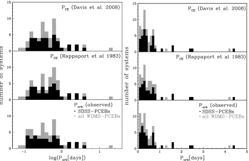
CE phase (PCE). The corresponding orbital period distributions are shown in Fig.1. As most of the observed PCEBs are rela-tively young and most of our PCEBs have low-mass secondary stars for which gravitational radiation is assumed to be the only sink of angular momentum, the reconstructed zero age post-CE distribution of orbital periods is not dramatically different from the observed distribution. In addition, the distributions of the systematically identified SDSS PCEBs (black histogram in Fig.1) do not differ significantly from the distribution of pre-viously known PCEBs that have been identified through various channels (Schreiber & Gänsicke 2003). In the following sections we use the zero-age PCEB parameter reconstructed with the dis-rupted magnetic braking prescription as given byHurley et al. (2002) and normalized byDavis et al.(2008). After reconstruct-ing the post-CE evolution, we can now concentrate on discussreconstruct-ing implications for theories of CE evolution that can be drawn from our sample.
4. CE equations
It is generally assumed that the outcome of the CE phase can be approximated by equating the binding energy of the envelope and the change in orbital energy, and by scaling this equation with an efficiencyα, i.e.
Egr=αΔEorb, (3)
whereEgris the gravitational (or binding) energy andΔEorb =
Eorb,i−Eorb,f is the total change in orbital energy during the CE phase. A variety of slightly different expressions forEorb,i,Eorb,f, andEgr appeared in the literature and we briefly review them here.
The final orbital energyEorb,f is always calculated as the or-bital energy between the core of the primary (M1,c) and the sec-ondary (M2) at the final separation (af)
Eorb,f = 1 2
GM1,cM2
af ·
(4)
In contrast, different descriptions exist for the gravitational en-ergy and the initial orbital enen-ergy. Some authors (e.g.Webbink 1984; de Kool 1990; Podsiadlowski et al. 2003) calculate the gravitational energy as being between the envelope mass (M1,e) and the mass of the primary (M1)
Egr=
GM1M1,e
λR , (5)
whereλdepends on the structure of the primary star, and the initial orbital energy as the orbital energy between the primary and the secondary at the initial separation (ai)
Eorb,i= 1 2
GM1M2
ai
· (6)
As inKiel & Hurley(2006), we will refer to this as the PRH (Podsiadlowski-Rappaport-Han) formulation.
Another formulation (e.g. Iben & Livio 1993; Yungelson et al. 1994) takes the binding energy as being between the en-velope mass and the combined mass of the core of the primary and the secondary star
Egr=
G(M1,c+M2)M1,e 2ai
Fig. 1.Observed, present-day (bottom) and reconstructed post-CE (middleandtop) orbital period distributions (left: logarithmic scale,right: linear scale) for two different prescriptions of magnetic braking. The well-defined sample of SDSS-PCEBs is shown in black while the gray distribution represents the entire WDMS PCEB population (IK Peg is not present in the right panel of this figure due to its long period compared with the rest of the sample). There is no significant difference between the two populations. The observed distributions as well as the reconstructed zero-age PCEB distributions show a strong peak at∼8 h and a secondary peak at∼17 h. The reconstructed distributions for both prescriptions of disrupted magnetic braking are very similar because most PCEBs are relatively young and/or contain fully convective secondary stars.
and the initial orbital energy as the orbital energy between the core of the primary and the secondary at the initial binary sepa-ration
Eorb,i= 1 2
GM1,cM2
ai ·
(8) We will refer to this as the ILY (Iben-Livio-Yungelson) formu-lation.
Finally there is another scheme, used in the binary star evolu-tion (hereafter BSE) code presented byHurley et al.(2002), that takes the gravitational energy in the same way as in the PRH for-mulation (Eq. (5)) and the initial orbital energy as in the ILY for-mulation (Eq. (8)). We will refer to this as the BSE formulation. We compare the results obtained with the three formulations in Sect.6.
5. The reconstruction algorithm
As in NT05, we determined the possible masses and radii of the progenitors of the WDs in all the PCEBs listed in TablesA.1 andA.2 from fits to detailed stellar-evolution models. We as-sumed that the observed WD mass (MWD) is equal to the core mass of the giant progenitor (M1,c) at the onset of mass trans-fer and used the equations fromHurley et al.(2000) to calcu-late the luminositiesLg an radiiRg of all giant stars that have
exactly such a core mass. We did this for initial massesM1 of 1.0,1.01,1.02, ...Mup to the mass for which the initial core mass, i.e. the core mass at the end of the main sequence, is larger than the observed WD mass. We also included possible progen-itors in the Hertzsprung gap (HG) with initial masses greater than 1.2M(to ensure a convective envelope). Because we used equations fromHurley et al.(2000) for the different evolutionary stages instead of running the code, we set mass dependent lumi-nosity limits for the progenitors in different evolutionary phases. For stars in the HG we required the luminosity to be between the luminosity at the top of the main sequence and the luminosity at the base of the first giant branch (FGB) (i.e.LTMS≤Lg ≤LBGB). For the FGB, the luminosity should be between the luminos-ity at the base and at the end of the FGB phase respectively (i.e.LBGB ≤Lg ≤ LHeI). For the early asymptotic giant branch (EAGB), we required the luminosity to be between the lumi-nosity at the base of the AGB and the lumilumi-nosity of the second dredge-up (i.e.LBAGB≤Lg≤LDU). Finally, for the second AGB (SAGB, i.e. after the second dredge-up) we required the lumi-nosity to be lower than the peak lumilumi-nosity of the first thermal pulse according to Eq. (29) inIzzard et al.(2004). For all possi-ble progenitors we also requiredq= M1/M2 to be greater than a critical value (qcrit), neccessary to have a CE according toTout
After obtaining the mass and radius of a possible WD pro-genitor with a core mass equal to the measured WD mass, we assumed that the giant radius was equal to the Roche-lobe radius at the onset of mass transfer. Because the secondary mass is as-sumed to remain constant during the CE phase, this allows us to determine the orbital separation just before the CE phase. The re-maining quantities in the CE equation are then the CE efficiency
αand the binding energy parameterλ, and we can derive αλ for each possible progenitor. In other words, from Roche geom-etry and the energy equation, we get one value forαλfor each parameter set consisting of the progenitor mass, core mass (= current WD mass), secondary mass (=current secondary mass), and final orbital period (=PCE). In this way we obtain a range of values forαλfor each system that corresponds to a range of possible progenitor massesM1.
6. Comparing CE prescriptions
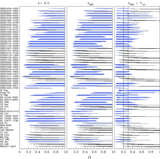
Before discussing below what we might be able to learn from reconstructing the new and much larger sample of PCEBs, we compare here the results obtained with the three formulations used to describe the CE evolution (Sect.4). Each horizontal line in Fig.2represents possible values ofαλfor different masses of the progenitor for a given WD and secondary mass. As in NT05, the different lines for each object represent different values of the WD mass within 0.05Mfrom the best-fit value (or within the error given in TableA.1andA.2in case it exceeds 0.05M). Values obtained for FGB progenitors are shown in black, while AGB progenitors are in blue (see the electronic version of the pa-per for a color version). We did not find any possible progenitor on the HG phase.
Solutions for most of the non-SDSS PCEBs are also given in NT05 (their Fig. 6). Comparing their results with those shown in the left panel of Fig.2one finds that the two reconstruction algorithms give very similar results with the only notable diff er-ence that we generally find slightly more solutions for a given system. This is because our grid of progenitor masses is finer by a factor of ten (step size 0.01Minstead of 0.1M).
Comparing the three panels of Fig.2it becomes obvious that the results obtained with the PRH and BSE algorithm are almost identical, withαλbeing a little but not significantly lower for the BSE scheme. There are, however, significant differences be-tween those two formulations and the ILY scheme, which gives by far the lowest values. This is easy to understand as the ILY formulation predicts much lower values for the gravitational en-ergy than the PRH prescription. We also note that the ILY ver-sion ofEgr does not contain the structural parameterλ. Hence, we are in fact plottingαfor this formulation. In general, it is dif-ficult – if not impossible – to judge which of the three algorithms for the initial conditions of CE evolution should be used. In any case, much of the physics is contained in the parametersαandλ. As most calculations presented in the literature are based on the PRH or the BSE formalism, we will use the BSE formulation in the following sections to facilitate the comparison of our results with those obtained by other authors.
7. The binding energy of the envelope
The structural parameterλhas generally been taken as a constant (typically∼0.5). Detailed stellar models taking into account the structure of the envelope show that this is a reasonable assump-tion as long as the internal energy of the envelope is ignored. In this case one obtainsλ ∼ 0.2−0.8. However, according to e.g.
Dewi & Tauris(2000);Podsiadlowski et al.(2003),λ = 0.5 is not a very realistic assumption if a fraction of the internal energy of the envelope supports the process of envelope ejection. In this case, especially the extended envelopes of luminous AGB stars can be very loosely bound, i.e. reaching values ofλ10. This is mainly due to the recombination-energy term. It is still not entirely clear whether this energy indeed contributes to unbind the envelope of the donor or if it is entirely radiated away (see e.g.Soker & Harpaz 2003;Han et al. 2003, for further discus-sion). However, the internal energy of the envelope might be a very important factor to explain the existence of long orbital pe-riod systems, and we therefore followHan et al.(1995), who introduced a parameterαth (between 0 and 1) to characterize the fraction of the internal energy that is used to expell the CE. Using this, and calling the parameterαint(as it includes not only the thermal energy, but also the radiation and the recombination energy), the equation for the standardα-formalism becomes
αorbΔEorb=Egr−αintUint. (9)
Alternatively one can reviseλto incorporate the internal energy Uint. If a fraction of the internal energy contributes to expelling the envelope, the binding energy writes
Ebind=
M1
M1,c
−Gm
r(m)+αintUint(m) dm. (10) Detailed calculations of this expression have been performed by various authors (e.g.Dewi & Tauris 2000;Podsiadlowski et al. 2003) who demonstrate that the binding energy depends signif-icantly on the mass of the giant, its evolutionary state, and of course,αint. Clearly, to include the effect of the internal energy and the structure of the envelope in the simple energy equation (Eq. (3)) one may equateEbindwith the parametrized binding en-ergyEgrfrom Eq. (5), keepingλvariable. The latest version of the BSE code includes an algorithm that computesλin this way. Ebindhas been calculated using detailed stellar models fromPols
et al.(1998) and approximated with analytical fits (Pols, priv. commun.). Using this algorithmλis no longer a constant but de-pends on the mass, the evolutionary state of the mass donor, and on the fraction of the internal energy used to expel the envelope, i.e.αint. Note that the exact definition of the core radius that sep-arates the ejected envelope from the condensed core region in the primary is of major importance for high-mass progenitors on the FGB (Tauris & Dewi 2001;van der Sluys et al. 2006). As we mostly find low-mass progenitors on the FGB the exact def-inition of the core radius (and hence of the core mass) can be assumed to be of minor importance here.The prescription ofλ used in this work is based on the core-envelope boundary be-ing defined as the mass shell where the hydrogen mass fraction becomes less than 10%.
In the next sections we assume the efficiency of using the internal energy of the envelope and the orbital energy to expell the envelope to be equal, i.e. we use values ofλthat include a fractionαint = αorb = α. Hence, the given values ofαshould be interpreted as the fraction of the total energy that is used to expell the envelope, independent of whether this energy has to be transferred from the orbit to the envelope or was already present in the envelope as internal energy.
is hardly any difference between the black lines in the three pan-els. However, the effect of calculatingλand including the in-ternal energy is of utmost importance for AGB progenitors: the blue lines move towards lower values ofαespecially if a frac-tion of the internal energy is assumed to contribute to the energy budget of CE evolution. The effect is most obvious for IK Peg because we only find a solution with 0 ≤α ≤1 if the internal energy is included. This result perfectly agrees withDavis et al. (2010). In addition, the internal energy becomes important espe-cially for long orbital period systems – exactly as suggested by Webbink(2008).
Inspecting the right panel of Fig. 3 in more detail, it be-comes obvious that including the internal energy allows us to find solutions for all the systems in a small range of CE effi cien-cies, i.e.α = 0.2−0.3 (vertical lines). The upper limit of this range (α=0.3) is defined by systems with massive WD (so they have progenitors on the AGB) and short orbital periods after the CE phase. In contrast, the lower limit (α=0.2) is given by sys-tems with FGB progenitors (i.e. those with low-mass WDs).
8.
α
versusγ
As mentioned above, NT05 used a similar algorithm to recon-struct the CE phase of double WDs and PCEBs. The problem they encountered can be summarized as follows: during the first CE phase of virtually all double WDs and for three alleged PCEBs (AY Cet, S1040 and IK Peg) the observed binary separa-tion is too large, requiring a physically unrealisticly high or even a negative efficiency. NT05 therefore proposed to use the angu-lar momentum conservation instead of the energy conservation because they find the angular momentum relation in agreement with the observed binary separations of double WDs and all the PCEBs in their sample. The alternative angular momentum algo-rithm for CE evolution (the so calledγ-algorithm) is described by
ΔJ
J =γ ΔMtotal
Mtotal =γ
M1,e
M1+M2,
(11)
whereΔJJis the relative change in angular momentum andΔMtotal
Mtotal
is the relative change in mass. At first glance, the fact that all the unexplained double WDs and the three alleged critical PCEBs have reasonable solutions forγ appears to be very attractive. Moreover, the obtained values ofγcluster in a rather small range of values, i.e. 1.5 ≤γ ≤ 1.75, raising hope for a new and uni-versal prescription of CE evolution. However, this turned out to be an illusion asWebbink(2008) recently showed that energy conservation is much more constraining the outcome of CE evo-lution. Indeed, a final energy state lower than the initial one re-quires the loss of angular momentum while the opposite is not necessarily true. In addition,Webbink (2008) showed that the ratio of final to initial orbital separation is extremely sensitive to
γin the range of values proposed by NT05.
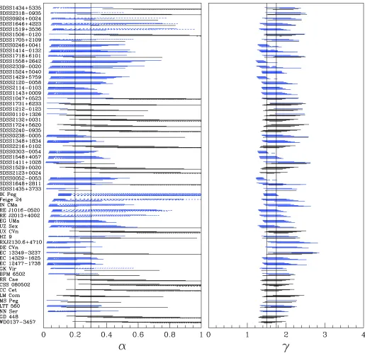
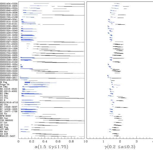
Our large and representative sample of PCEBs now allows us to test both algorithms and to evaluate their predictive power. In Fig.4we show the values ofα(left) andγ(right) for all possi-ble progenitors of the PCEBs in our sample. The binding energy parameterλhas been calculated with the BSE code including internal energy. All the PCEBs in our sample can be simulta-neously reproduced withαin the range 0.2−0.3 (vertical lines in the left panel). The right panel shows that indeed literally all systems can be reconstructed withγ=1.5−1.75 (vertical lines). In Fig.5 we investigate the effect of constrainingαon the possible range of values forγand vice versa. In the left panel
we show the values ofαrequesting 1.5 < γ < 1.75, while on the right hand side we show the values ofγif 0.2 ≤ α ≤ 0.3. Apparently, requestingγto lie in a small range of values does not very much constrain the values obtained forα. We still find the solutions forαcovering basically the entire parameter space, i.e. 0< α <1. This confirms the suggestion ofWebbink(2008) that virtually all possible configurations can be explained with similar values ofγ, which questions the predictive power of the new algorithm.
In contrast to this, fixingαprovides strong constraints onγ. The values we obtain forγseem to have a clear dependency on the evolutionary stage of the WD progenitor. It is almost constant for progenitors in the same evolutionary stage, being higher for FGB progenitors and smaller for AGB progenitors. This finding has a straightforward physical interpretation: the envelope of a giant star is more tightly bound on the FGB and less bound on the AGB, where it is more expanded (especially on the second AGB). The value ofγrepresents the ratio of the relative amount of angular momentum loss to the relative amount of mass loss. Hence, the different values ofγmay just reflect the simple fact that expelling a tightly (loosely) bound envelope requires to ex-tract more (less) angular momentum per unit mass.
Once more, the findings described above perfectly agree with the results obtained byWebbink (2008), i.e. we need to con-strain α to predict the outcome of CE evolution. In addition, the internal energy of the envelope seems to play an important role. Taking this into account in the energy equation leads to two classes of solutions in the angular momentum equation.
9. Should
α
be constant?In most binary population synthesis models of WDMS (e.g. Willems & Kolb 2004) but also of soft X-ray transients (Yungelson & Lasota 2008; Kiel et al. 2008) or extreme hori-zontal branch stars (Han et al. 2002), the CE efficiency is as-sumed to be constant. Analyzing our sample of PCEBs consist-ing of WDs and low-mass main-sequence stars we find that we can reconstruct the evolutionary history of all systems assuming a constant valueα∼ 0.2−0.3.
An important question is now whether we should expectα to be constant for all types of PCEBs. First steps exploring this have been made byPolitano & Weiler(2007),Davis et al.(2008, 2010) who recently speculated that instead of being constant,α may depend on the mass of the secondary star or on the final orbital separation as spiraling-in deeper into the envelope may significantly affect the efficiency of the ejection process.
We here followDavis et al.(2008) and evaluate the forma-tion probability for each possible progenitor of each PCEB in our sample. The number of primaries with masses in the range dM1 is given by dN ∝ f(M1)dM1 where f(M1) is given by the initial mass function (IMF):
f(M1)=
⎧⎪⎪ ⎪⎪⎪⎨ ⎪⎪⎪⎪⎪ ⎩
0 M1/M<0.1, 0.29056M−1.3
1 0.1≤M1/M<0.5, 0.15571M−2.2
1 0.5≤M1/M<1.0, 0.15571M−2.7
1 1.0≤M1/M,
(12)
(Kroupa et al. 1993). The probability that a binary forms with a certain initial orbital separationaiis determined by
h(ai)=
0 ai/R<3 orai/R>106,
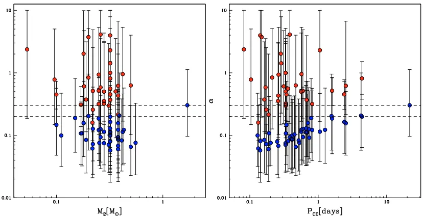
Fig. 6.Weighted mean values ofαversusM2(left) andPCE(right). Red is for systems with FGB progenitors, while blue is for AGB progenitors. The full range of possible values ofαis given by the solid vertical lines. Dashed horizontal lines are forα=0.2 and 0.3.
In Fig.6we plot the weighted mean value ofαfor each sys-tem (colored points) versus the mass of the secondary star (left) and the orbital period the PCEB had at the end of the CE phase (right). Black vertical lines represent the full range of possible values ofα. Again, we distinguish between progenitors in diff er-ent evolutionary stages. Red points indicate systems with pro-genitors on the FGB, while blue points are for propro-genitors on the AGB. Given the uncertainties in the WD masses, some sys-tems have possible progenitors in more than one evolutionary stage. For those cases, we separately computed the average for the different type of progenitors. Finally, dashed horizontal lines indicateα =0.2 and 0.3. There seems to be no dependence of
αon the mass of the secondary star or on the period, but a large scatter aroundα=0.2−0.3.
This finding remains if we assume alternative initial mass distributions. We tested for two other probability distributions assuming that the masses of the binary components are corre-lated. We used n(q2) ∝ q2 and n(q2) ∝ q−20.99, where q2 =
M2/M1. In both cases we obtained very similar results, i.e., a large scatter and no relation betweenαandM2orPCE. Although there seems to be no correlation betweenαand the mass of the secondary or the final period, there is a clear relation between the averaged mean values ofαand the evolutionary state of the pro-genitor. Systems with FGB progenitors tend to have weighted mean valuesα > 0.3, while the obtained mean efficiencies for systems with AGB progenitors are much smaller, i.e.α 0.1. This is easily explained if one remembers that the internal en-ergy becomes very important for progenitors on the AGB mov-ing the whole range of possible values ofαtowards smaller val-ues (see Sect.7). It is essential to recall here that the given values ofα represent the fraction of the total energy that is used to expell the envelope. In other words, the same fraction of in-ternal and orbital energy are used, i.e.αint = α. However, one could also point out that the orbital energy must first be trans-ferred to the envelope (presumably as thermal energy), in con-trast to the energy already present in the envelope and that this would give rise to a differentαfor the two. Indeed, the system-atically lower weighted mean values ofαfor AGB progenitors may reflect different efficiencies for the orbital and internal en-ergy. Ifαintis small, the requiredαorbwill increase especially for
systems with AGB progenitor. So, an alternative toα = const. might beαorb=const andαint=const butαint< αorb. A detailed discussion of this alternative possibility is beyond the scope of this paper though.
As a final remark we emphasize that the weighted mean val-ues discussed above are lacking a physical meaning. We used these values here only to test for possible dependencies ofαthat are missing in the energy equation, which does not seem to be the case. Therefore, α = const. or at least αorb = const. and
αint=const., which corresponds to the assumption that the most important dependencies are included in the used energy equation remains the currently most reasonable prescription.
10. Discussion
The results obtained in the previous sections can be summarized as follows: For all systems in our sample, which is the largest sample of one specific type of PCEBs that is currently avail-able, we find possible progenitors assuming energy conservation if the internal energy of the envelope is taken into account. For each individual system the possible solutions cover rather broad ranges of values for the CE efficiencyα. However, there exists only a small range of values, i.e.α=0.2−0.3 for which we find solutions for all the systems in our sample. This means that, if a universal value for the CE efficiency does exist, it should lie in this range. A plausible alternative to such a universal value forαis to assume that the fraction of the orbital energy exceeds the fraction of the internal energy that is used to expell the enve-lope, i.e.αint< αorb. In addition, we have shown that the energy budget constrains the outcome of CE evolution much more than the alternative angular momentum equation. In this section we discuss our results in the context of recent theoretical and ob-servational results in the field of close compact binary formation and evolution.
10.1. Hydrodynamical simulations
were carried out (Taam et al. 1978;Meyer & Meyer-Hofmeister 1979). Based on these early studies two and three dimen-sional models have been developed in the last decades (e.g. Bodenheimer & Taam 1984; Taam & Bodenheimer 1989; Sandquist et al. 2000). For a recent review see e.g. Taam & Ricker(2006). The most important findings of hydrodynamical simulations of CE evolution are perhaps the relatively short du-ration of CE evolution (1000 yrs) and the preference of ejecting matter in the orbital plane. In addition, as most particles are pre-dicted to leave the CE with velocities exceeding the minimum escape speed, the predicted CE efficiency is less than 40−50%, i.e.α 0.4−0.5. This result agrees quite well with our finding ofα=0.2−0.3. However, one should note that current hydrody-namical simulations still cannot follow the entire CE evolution basically because of the large ranges of timescales and length scales that have to be numerically resolved. Therefore, even the most detailed hydrodynamical simulations still have to be con-sidered as rather rough approximations.
10.2. Binary population synthesis
An alternative way to constrain the CE efficiency is to perform binary population studies and compare the predictions with the observed properties of PCEBs. These simulations have become popular in last 10−20 years and have been carried out for a large variety of different PCEB populations. We here briefly review the main results.
10.2.1. WDMS binaries
The population of WDMS binaries has been first simulated by de Kool(1992) andde Kool & Ritter(1993).de Kool & Ritter (1993) incorporated observational selection effects to compare their predictions with the – very small and biased – observed populations they had at hand. Interestingly, forα = 0.3 and M2randomly taken from the IMF they predict PCEB orbital pe-riod distributions rather similar to the observed distribution (see Sect. 3). However, the selection effects applied by de Kool & Ritter (1993) have been designed for blue color surveys such as the Palomar Green survey and are not applicable to our new SDSS PCEB sample. In addition, one should take into account that the approximations to stellar evolution used byde Kool & Ritter(1993) have been much cruder than the models that are available today and that they did not include the internal energy of the envelope.
An update of this early work was carried out byWillems & Kolb(2004), using more detailed analytical fits to stellar evo-lution (Hurley et al. 2000). Their PCEB orbital period distri-bution peaks at about one day, i.e. at a significantly longer pe-riod than the observed sample. However, one should note that Willems & Kolb(2004) computed formation models for PCEBs, but did not follow the subsequent angular momentum loss by magnetic braking and gravitational radiation. In addition, no ob-servational biases are incorporated in their preditions. Hence, we advocate caution when comparing the predictions ofWillems & Kolb(2004) with observed samples.
Full binary population studies of PCEBs have been per-formed byPolitano & Weiler(2006,2007). They tested different formulations ofαand discussed the influence on the predicted distributions. The resulting orbital period distributions peak at Porb ∼ 3 days and the overall shape does not change signifi-cantly for different prescriptions of the CE efficiency. Again, as observational selection effects have not been incorporated, it is
difficult, if not impossible, to compare the predicted distributions with the measured orbital period distributions shown in Fig.1.
Most recently, Davis et al. (2010) published a work pre-senting comprehensive population synthesis studies of PCEBs. Perhaps most importantly, for the first time the PCEB population has been simulated including variable values ofλ. Comparing their predictions with the observations,Davis et al.(2010) find a disagreement in the orbital period distributions, i.e. the pre-dicted distributions peak atPorb ∼ 1 day declining smoothly at longer periods, while observations indicate a rather steep decline atPorb∼ 1 day. However,Davis et al.(2010) compared their pre-dictions with a small sample of PCEBs identified through vari-ous detection channels. Thanks to our concentrated follow-up of WDMS binaries from SDSS, the number of known PCEBs has increased by more than a factor of two, and this new SDSS PCEB sample is less affected by observational biases (Gänsicke et al. 2010, in prep). In addition, the parameter space explored byDavis et al. (2010) is still rather small. While the CE effi -ciency has in general been varied over a wide range of values (α=0.1−1), only one model with variable values ofλassuming
α=1 has been calculated. Finally, one should keep in mind that Davis et al.(2010) interpolated the tables provided byDewi & Tauris(2000) to determineλ, which probably leads to underes-timatingλfor large radii.
We conclude that binary population synthesis (BPS) simu-lations usingα = αint =0.2−0.3 and including a proper treat-ment ofλdo not yet exist. Hence, it might not be too surprising that predicted period distributions disagree with the observation. Reducingαand incorporating the internal energy should lead to predicting less systems withPorb≥ 1 day. Therefore we antici-pate that applying our results may bring theory and observations into agreement. In addition, the next generation of BPS simula-tions should take into account observational biases as detailed as possible. The importance of this might be indicated by the basic agreement between the predictions byde Kool & Ritter(1993) and our observed sample.
10.2.2. Extreme horizontal branch stars
Extreme horizontal branch stars (EHB, also known as hot sub-dwarfs) are helium-burning stars with very thin hydrogen en-velopes (Heber et al. 1986;Saffer et al. 1994). To explain the formation of these stars several scenarios have been discussed mostly based on single-star evolution (e.g.Kilkenny et al. 1997; Green et al. 1986). However, as most EHB stars appear to be members of close binary systems, the binary-formation chan-nel proposed byHan et al.(2002,2003) has become a popu-lar alternative. These authors favored a rather high efficiency (α ∼ 0.75) when compared to the value we obtain from our sample. However, one should note thatHan et al.(2003) did not explore the full parameter space and did not generally exclude lower values ofα.
fractions among EHB stars in globular clusters are required to derive clear constraints.
10.2.3. Low-mass X-ray binaries
The efficiency of CE evolution is of outstanding importance in the context of compact binaries descending from more massive stars too. For example, the existence of low-mass X-ray bina-ries (LMXBs) in our galaxy has been difficult to explain within the CE picture as low-mass companions appear to be unable to unbind the envelope of a massive primary star (Podsiadlowski et al. 2003) and one therefore expects most systems to merge instead of forming a LMXB. As shown byPodsiadlowski et al. (2003), the predicted formation rate of LMXBs is much lower than indicated by observations even for α = 1. This is ex-plained by the huge binding energy of envelopes around mas-sive cores, i. e.λ 0.1. As a solution for this problem,Kiel & Hurley(2006) proposed a reduced mass-loss for helium stars and brought into agreement binary populations synthesis and ob-servations forα∼ 1.0 (but see alsoYungelson & Lasota 2008). In any case, current models seem to be unable to reproduce the observed population of LMXBs assuming a rather low value of
α=0.2−0.3 as we find for our sample of PCEBs. This indicates that either the efficiency is different for LMXBs or that the uncer-tainties in evolutionary models of very massive late AGB stars strongly affect the predictions of BPS.
11. Conclusion
We have developed a new algorithm to reconstruct CE evolution of PCEB stars. We included a proper treatment of the binding energy parameterλ taking into account the internal energy of the envelope. We have applied the new algorithm to the largest and most homogeneous sample of PCEBs currently available. The basic result of this investigation can be summarized with the following four statements:
– A reasonable prescription of the CE evolution of PCEBs con-taining a WD primary and late-M spectral-type secondary is given by the energy equation if the internal energy of the en-velope is included.
– The energy equation is much more constraining the outcome of CE evolution and the predictive power of the angular mo-mentum equation is limited.
– If there is a universal value ofα, it must be in the range of 0.2−0.3.
– There are no indications for a dependence ofαon the mass of the secondary star or the orbital period.
Despite these findings, it is still unclear whether a universal con-stant value ofαcan explain CE evolution in general. Answering this question requires to observationally establish representative and large samples of all types of PCEBs, i.e. not only WDMS, but also neutron star/black hole PCEBs. However, if such a value exists, our result ofα=0.2−0.3 can be interpreted as a defini-tive answer to one of the important questions in close compact binary evolution, especially as there seems to be no dependence of the CE efficiency on the mass of the secondary star or the final orbital period.
Acknowledgements. M.Z. is supported by an ESO studentship. MRS acknowl-edges support from FONDECYT (grant 1061199). We thank the referee, Marc van der Sluys, for helpfull comments.
References
Abazajian, K. N., Adelman-McCarthy, J. K., Agüeros, M. A., et al. 2009, ApJS, 182, 543
Adelman-McCarthy, J. K., Agüeros, M. A., Allam, S. S., et al. 2008, ApJS, 175, 297
Althaus, L. G., & Benvenuto, O. G. 1997, ApJ, 477, 313
Bergeron, P., Wesemael, F., Beauchamp, A., et al. 1994, ApJ, 432, 305 Bleach, J. N., Wood, J. H., Catalán, M. S., et al. 2000, MNRAS, 312, 70 Bodenheimer, P., & Taam, R. E. 1984, ApJ, 280, 771
Bragaglia, A., Renzini, A., & Bergeron, P. 1995, ApJ, 443, 735
Burleigh, M. R., Hogan, E., Dobbie, P. D., Napiwotzki, R., & Maxted, P. F. L. 2006, MNRAS, 373, L55
Davis, P. J., Kolb, U., Willems, B., & Gänsicke, B. T. 2008, MNRAS, 389, 1563 Davis, P. J., Kolb, U., & Willems, B. 2010, MNRAS, 403, 179
de Kool, M. 1990, ApJ, 358, 189 de Kool, M. 1992, A&A, 261, 188
de Kool, M., & Ritter, H. 1993, A&A, 267, 397
DeGennaro, S., von Hippel, T., Winget, D. E., et al. 2008, AJ, 135, 1 Dewi, J. D. M., & Tauris, T. M. 2000, A&A, 360, 1043
Drake, A. J., Djorgovski, S. G., Mahabal, A., et al. 2009, ApJ, 696, 870 Fulbright, M. S., Liebert, J., Bergeron, P., & Green, R. 1993, ApJ, 406, 240 Green, R. F., Richstone, D. O., & Schmidt, M. 1978, ApJ, 224, 892 Green, R. F., Schmidt, M., & Liebert, J. 1986, ApJS, 61, 305 Guinan, E. F., & Sion, E. M. 1984, AJ, 89, 1252
Han, Z. 2008, A&A, 484, L31
Han, Z., Podsiadlowski, P., & Eggleton, P. P. 1994, MNRAS, 270, 121 Han, Z., Podsiadlowski, P., & Eggleton, P. P. 1995, MNRAS, 272, 800 Han, Z., Podsiadlowski, P., Maxted, P. F. L., Marsh, T. R., & Ivanova, N. 2002,
MNRAS, 336, 449
Han, Z., Podsiadlowski, P., Maxted, P. F. L., & Marsh, T. R. 2003, MNRAS, 341, 669
Heber, U., Kudritzki, R. P., Caloi, V., Castellani, V., & Danziger, J. 1986, A&A, 162, 171
Hillwig, T. C., Honeycutt, R. K., & Robertson, J. W. 2000, AJ, 120, 1113 Hjellming, M. S. 1989, Ph.D. Thesis, A&A (Illinois Univ. Urbana-Champaign,
Savoy)
Hurley, J. R., Pols, O. R., & Tout, C. A. 2000, MNRAS, 315, 543 Hurley, J. R., Tout, C. A., & Pols, O. R. 2002, MNRAS, 329, 897 Iben, I. J., & Livio, M. 1993, PASP, 105, 1373
Izzard, R. G., Tout, C. A., Karakas, A. I., & Pols, O. R. 2004, MNRAS, 350, 407 Kawka, A., Vennes, S., Dupuis, J., & Koch, R. 2000, AJ, 120, 3250
Kawka, A., Vennes, S., Dupuis, J., Chayer, P., & Lanz, T. 2008, ApJ, 675, 1518 Kepler, S. O., & Nelan, E. P. 1993, AJ, 105, 608
Kiel, P. D., & Hurley, J. R. 2006, MNRAS, 369, 1152
Kiel, P. D., Hurley, J. R., Bailes, M., & Murray, J. R. 2008, MNRAS, 388, 393 Kilkenny, D., O’Donoghue, D., Koen, C., Stobie, R. S., & Chen, A. 1997,
MNRAS, 287, 867
Knigge, C. 2006, MNRAS, 373, 484
Koester, D., Schulz, H., & Weidemann, V. 1979, A&A, 76, 262 Kroupa, P., Tout, C. A., & Gilmore, G. 1993, MNRAS, 262, 545 Landsman, W., Simon, T., & Bergeron, P. 1993, PASP, 105, 841 Lanning, H. H., & Pesch, P. 1981, ApJ, 244, 280
Marsh, T. R. & Duck, S. R. 1996, MNRAS, 278, 565
Maxted, P. F. L., Marsh, T. R., Moran, C., Dhillon, V. S., & Hilditch, R. W. 1998, MNRAS, 300, 1225
Maxted, P. F. L., Marsh, T. R., Morales-Rueda, L., et al. 2004, MNRAS, 355, 1143
Maxted, P. F. L., O’Donoghue, D., Morales-Rueda, L., Napiwotzki, R., & Smalley, B. 2007, MNRAS, 376, 919
Meyer, F., & Meyer-Hofmeister, E. 1979, A&A, 78, 167
Moni Bidin, C., Moehler, S., Piotto, G., et al. 2006, A&A, 451, 499 Moni Bidin, C., Catelan, M., & Altmann, M. 2008, A&A, 480, L1
Moni Bidin, C., Moehler, S., Piotto, G., Momany, Y., & Recio-Blanco, A. 2009, A&A, 498, 737
Nebot Gómez-Morán, A., Schwope, A. D., Schreiber, M. R., et al. 2009, A&A, 495, 561
Nelemans, G., & Tout, C. A. 2005, MNRAS, 356, 753
Nelemans, G., Verbunt, F., Yungelson, L. R., & Portegies Zwart, S. F. 2000, A&A, 360, 1011
O’Brien, M. S., Bond, H. E., & Sion, E. M. 2001, ApJ, 563, 971 O’Donoghue, D., Koen, C., Kilkenny, D., et al. 2003, MNRAS, 345, 506 Orosz, J. A., Wade, R. A., Harlow, J. J. B., et al. 1999, AJ, 117, 1598
Paczy´nski, B. 1976, in Structure and Evolution of Close Binary Systems, IAU Symp., 73, 75
Parsons, S. G., Marsh, T. R., Copperwheat, C. M., et al. 2010, MNRAS, 402, 2591
Politano, M., & Weiler, K. P. 2006, ApJ, 641, L137 Politano, M., & Weiler, K. P. 2007, ApJ, 665, 663
Pols, O. R., Schroder, K.-P., Hurley, J. R., Tout, C. A., & Eggleton, P. P. 1998, MNRAS, 298, 525
Pyrzas, S., Gänsicke, B. T., Marsh, T. R., et al. 2009, MNRAS, 394, 978 Rappaport, S., Joss, P. C., & Verbunt, F. 1983, ApJ, 275, 713
Rebassa-Mansergas, A., Gänsicke, B. T., Rodríguez-Gil, P., Schreiber, M. R., & Koester, D. 2007, MNRAS, 382, 1377
Rebassa-Mansergas, A., Gänsicke, B. T., Schreiber, M. R., et al. 2008, MNRAS, 390, 1635
Rebassa-Mansergas, A., Gänsicke, B. T., Schreiber, M. R., Koester, D., & Rodríguez-Gil, P. 2010, MNRAS, 402, 620
Saffer, R. A., Wade, R. A., Liebert, J., et al. 1993, AJ, 105, 1945 Saffer, R. A., Bergeron, P., Koester, D., & Liebert, J. 1994, ApJ, 432, 351 Sandquist, E. L., Taam, R. E., & Burkert, A. 2000, ApJ, 533, 984
Schmidt, G. D., Smith, P. S., Harvey, D. A., & Grauer, A. D. 1995, AJ, 110, 398 Schreiber, M. R., & Gänsicke, B. T. 2003, A&A, 406, 305
Schreiber, M. R., Nebot Gomez-Moran, A., & Schwope, A. D. 2007, in ASP Conf. Ser. 372, ed. A. Napiwotzki, & M. R. Burleigh, 459
Schreiber, M. R., Gänsicke, B. T., Southworth, J., Schwope, A. D., & Koester, D. 2008, A&A, 484, 441
Schreiber, M. R., Gänsicke, B. T., Rebassa-Mansergas, A., et al. 2010, A&A, 513, L7
Schwope, A. D., Nebot Gomez-Moran, A., Schreiber, M. R., & Gänsicke, B. T. 2009, A&A, 500, 867
Soker, N., & Harpaz, A. 2003, MNRAS, 343, 456 Stauffer, J. R. 1987, AJ, 94, 996
Taam, R. E., & Bodenheimer, P. 1989, ApJ, 337, 849
Taam, R. E., & Ricker, P. M. 2006 [arXiv:astro-ph/0611043] Taam, R. E., Bodenheimer, P., & Ostriker, J. P. 1978, ApJ, 222, 269 Tappert, C., Gänsicke, B. T., Schmidtobreick, L., et al. 2007, A&A, 474, 205 Tappert, C., Gänsicke, B. T., Zorotovic, M., et al. 2009, A&A, 504, 491 Tauris, T. M., & Dewi, J. D. M. 2001, A&A, 369, 170
Tout, C. A., Aarseth, S. J., Pols, O. R., & Eggleton, P. P. 1997, MNRAS, 291, 732
Townsley, D. M., & Bildsten, L. 2003, ApJ, 596, L227 Townsley, D. M., & Gänsicke, B. T. 2009, ApJ, 693, 1007
van den Besselaar, E. J. M., Greimel, R., Morales-Rueda, L., et al. 2007, A&A, 466, 1031
van der Sluys, M. V., Verbunt, F., & Pols, O. R. 2006, A&A, 460, 209 Vennes, S., Thorstensen, J. R., & Polomski, E. F. 1999, ApJ, 523, 386 Webbink, R. F. 1984, ApJ, 277, 355
Webbink, R. F. 2008, in Astrophysics and Space Science Library, ed. E. F. Milone, D. A. Leahy, & D. W. Hobill, Astrophys. Space Sci. Libr., 352, 233
Willems, B., & Kolb, U. 2004, A&A, 419, 1057
Wood, M. A. 1995, in White Dwarfs, ed. D. Koester & K. Werner, LNP No. 443 (Heidelberg: Springer), 41
Yungelson, L. R. & Lasota, J.-P. 2008, A&A, 488, 257
Yungelson, L. R., Livio, M., Tutukov, A. V., & Saffer, R. A. 1994, ApJ, 420, 336
Appendix A: Data
Table A.1.Properties of the SDSS PCEBs.
Object P MWD M2 TWD tcool PCE Ref.
(d) (M) (M) (K) (Gyr) (d) SDSS1435+3733 0.126 0.505±0.025 0.218±0.028 12 392 0.275 0.133 1 SDSS1648+2811 0.131 0.630±0.520 0.320±0.060 13 432 0.284 0.142 2 SDSS0052−0053 0.114 1.220±0.370 0.320±0.060 16 111 0.421 0.143 3 SDSS2123+0024 0.149 0.310±0.100 0.200±0.080 13 279 0.000 0.149 4 SDSS1529+0020 0.165 0.400±0.040 0.260±0.040 14 148 0.300 0.170 3 SDSS1411+1028 0.167 0.520±0.110 0.380±0.070 30 419 0.009 0.188 4 SDSS1548+4057 0.185 0.646±0.032 0.174±0.027 11 835 0.416 0.191 1 SDSS0303−0054 0.134 0.912±0.034 0.253±0.029 8000 2.24 0.20 1 SDSS2216+0102 0.210 0.400±0.060 0.200±0.080 14 200 0.297 0.212 4 SDSS1348+1834 0.249 0.590±0.040 0.319±0.060 15 071 0.184 0.251 5 SDSS0238−0005 0.212 0.590±0.220 0.380±0.070 21 535 0.045 0.261 4 SDSS2240−0935 0.261 0.410±0.080 0.250±0.120 12 536 0.443 0.263 4 SDSS1724+5620 0.333 0.420±0.010 0.360±0.070 35 746 0.000 0.333 3 SDSS2132+0031 0.222 0.380±0.040 0.320±0.010 16 336 0.179 0.333 4 SDSS0110+1326 0.333 0.470±0.020 0.310±0.050 25 167 0.051 0.333 1 SDSS1212−0123 0.333 0.470±0.010 0.280±0.020 17 304 0.191 0.334 6 SDSS1731+6233 0.268 0.450±0.080 0.320±0.010 16 149 0.228 0.361 4 SDSS1047+0523 0.382 0.380±0.200 0.260±0.040 12 392 0.417 0.384 7 SDSS1143+0009 0.386 0.620±0.070 0.320±0.010 16 910 0.138 0.411 4 SDSS2114−0103 0.411 0.710±0.100 0.380±0.070 28 064 0.018 0.416 4 SDSS2120−0058 0.449 0.610±0.060 0.320±0.010 16 149 0.156 0.450 4 SDSS1429+5759 0.545 1.040±0.170 0.380±0.060 16 336 0.401 0.566 5 SDSS1524+5040 0.590 0.710±0.070 0.380±0.060 19 640 0.109 0.601 5 SDSS2339−0020 0.655 0.840±0.360 0.320±0.060 13 266 0.508 0.657 3 SDSS1558+2642 0.662 1.070±0.260 0.319±0.060 14 560 0.609 0.664 5 SDSS1718+6101 0.673 0.520±0.090 0.320±0.010 18 120 0.075 0.678 4 SDSS1414−0132 0.728 0.730±0.200 0.260±0.040 13 904 0.329 0.729 7 SDSS0246+0041 0.728 0.900±0.150 0.380±0.010 16 572 0.309 0.739 3 SDSS1705+2109 0.815 0.520±0.050 0.250±0.120 23 613 0.023 0.815 4 SDSS1506−0120 1.051 0.430±0.130 0.320±0.010 15 422 0.251 1.057 4 SDSS1519+3536 1.567 0.560±0.040 0.200±0.080 19 416 0.065 1.567 4 SDSS1646+4223 1.595 0.550±0.090 0.250±0.120 17 707 0.093 1.595 4 SDSS0924+0024 2.404 0.520±0.050 0.320±0.010 19 193 0.059 2.404 4 SDSS2318−0935 2.534 0.490±0.060 0.380±0.070 22 550 0.026 2.534 4 SDSS1434+5335 4.357 0.490±0.030 0.320±0.010 21 785 0.030 4.357 4
Table A.2.Properties of the previously known PCEBs.
Object Alt. Name P MWD M2 TWD tcool PCE Ref.
(d) (M) (M) (K) (Gyr) (d) WD0137-3457 0.080 0.390±0.035 0.053±0.006 16500 0.179 0.082 1 GD 448 HR Cam 0.103 0.410±0.010 0.096±0.040 19000 0.118 0.104 2, 3 NN Ser PG 1550+131 0.130 0.535±0.012 0.111±0.004 57000 0.001 0.130 4 LTT 560 0.148 0.520±0.120 0.190±0.050 7500 1.040 0.162 5 MS Peg GD 245 0.174 0.480±0.020 0.220±0.020 22170 0.027 0.174 6 LM Com PG 1224+309 0.259 0.450±0.050 0.280±0.050 29300 0.032 0.259 7 CC Cet PG 0308+096 0.284 0.390±0.100 0.180±0.050 26200 0.000 0.284 8 CSS 080502 0.149 0.350±0.040 0.320±0.000 17505 0.130 0.288 9, 10 RR Cae LFT 349 0.303 0.440±0.022 0.182±0.013 7540 2.037 0.313 11 BPM 6502 LTT 3943 0.337 0.500±0.050 0.170±0.010 21000 0.036 0.337 12, 13, 14 GK Vir PG 1413+015 0.344 0.510±0.040 0.100±0.000 48800 0.002 0.344 15, 16 EC 14329−1625 0.350 0.620±0.110 0.380±0.070 14575 0.220 0.421 17 EC 12477−1738 0.362 0.610±0.080 0.380±0.070 17718 0.113 0.402 17 DE CVn J 1326+4532 0.364 0.530±0.040 0.410±0.060 8000 0.895 0.518 18 EC 13349−3237 0.470 0.460±0.110 0.500±0.050 35010 0.000 0.470 17 RXJ2130.6+4710 0.521 0.554±0.017 0.555±0.023 18000 0.088 0.530 19
HZ 9 0.564 0.510±0.100 0.280±0.040 17400 0.086 0.564 20, 21, 22, 23 UX CVn HZ 22 0.570 0.390±0.050 0.420±0.000 28000 0.000 0.570 24
UZ Sex PG 1026+0014 0.597 0.650±0.230 0.220±0.050 19900 0.084 0.597 8, 25 EG UMa Case 1 0.668 0.640±0.030 0.420±0.040 13100 0.313 0.688 26 RE J2013+4002 0.706 0.560±0.030 0.180±0.040 49000 0.002 0.706 27, 28 RE J1016−0520 0.789 0.600±0.020 0.150±0.020 55000 0.002 0.789 27, 28 IN CMa J0720−3146 1.260 0.570±0.030 0.430±0.030 52400 0.002 1.260 27, 29 Feige 24 FS Cet 4.232 0.570±0.030 0.390±0.020 57000 0.001 4.232 30 IK Peg BD+18 4794 21.722 1.190±0.050 1.700±0.100 35500 0.027 21.722 29, 31
References.(1)Burleigh et al.(2006); (2)Marsh & Duck(1996), (3)Maxted et al.(1998); (4)Parsons et al.(2010); (5)Tappert et al.(2007); (6)Schmidt et al.(1995); (7)Orosz et al.(1999); (8)Saffer et al.(1993); (9)Drake et al.(2009); (10)Pyrzas et al.(2009); (11)Maxted et al.