A Spatio Temporal Point Process Model for Firemen Demand in Twente

(1)

University of Twente

A Spatio-Temporal Point Process Model

for Firemen Demand in Twente

Bachelor Thesis

Author:

Mike Wendels

Supervisor:

prof. dr. M.N.M. van Lieshout

Stochastic Operations Research

Applied Mathematics

(2)

A Spatio-Temporal Point Process Model for Firemen

Demand in Twente

Mike Wendels1

Department of Applied Mathematics, Chair Stochastic Operations Research, University of Twente, P.O. Box 217 NL-7500 AE Enschede, The Netherlands

31-3-2017

Abstract: In this thesis a spatio-temporal point process will be proposed for modelling firemen demanding emergency calls in the region Twente in the Netherlands. The modelling technique will be described for the level 1a classifications of firemen demanding emergency calls “fire”, “service”, “acci-dent”, “alert” and “environmental”. Making accurate expectations for these kinds of emergency calls in the future is very important for emergency ser-vices, since it can improve the prevention behaviour and the scheduling of the fire departments and therefore the quality of help. Improvement of the prevention behaviour is made possible because the model describes the influ-ences of the involved covariates on each class of emergency calls. Scheduling could be improved since the number of emergency calls with the correspond-ing locations and classes can be predicted for future days. In this way it can be predicted for every fire department how many and which kinds of emer-gency calls they will have to treat the next days. Nowadays these predictions are often made by the industry practice model of partitioning the region of interest in polygons and base the expected number of emergency calls on cor-responding information of the past by taking averages. But spatio-temporal point process models have proven to be the more accurate and robust model, since scientific research highly improved the theory for spatial point pattern analysis the last few decades. Spatial point process modelling has also be sim-plified by the many tools for analysing spatial point patterns available in the

spatstat package in R, available from CRAN (2006). This thesis provides extensions to some of these tools, because a spatio-temporal point process will be developed for the emergency calls rather than a purely spatial point process. This spatio-temporal point process actually involves an ensemble of spatio-temporal point processes for the emergency calls of each level 1a class and each of these models thus have to be modelled separately. These individ-ual spatio-temporal point processes will then be modelled as inhomogeneous Poisson processes for which the intensity function is dependent on spatial and temporal covariates. After modelling, the precise influences of each covariate involved on each kind of emergency calls will be known.

Key words: spatio-temporal point process, spatial point pattern, time series, inhomogeneous Poisson process, maximum pseudolikelihood estimator

1_Student _in _Applied _Mathematics _at _the _University _of _Twente, _Enschede, _The _Netherlands,

(4)

1 Introduction

Nowadays, emergency services base their logistics and prevention behaviour strongly on their expectations for the emergency calls in the future. Making these expectations as accurate as possible has been (and still is) a hot topic in scientific research. Because the better the pre-dictions of emergency calls are, the better emergency services can anticipate their logistics and prevention behaviour on it.

Every emergency call has a time t ∈ R+ and a location x ∈ R2 of occurrence. Mostly the description of emergency calls are completed with a classificationci, i∈N,of the emergency call, for example a description of the emergency call or the priority for serving the emergency call. Emergency services desire to know all the exact times, locations and the potential classifications of the future emergency calls, so they can serve aid on the right time, at the right location and with the right means. Creating a model which predicts these variables exactly for every future emergency call is of course a utopian aim. So each model will in some way involve stochastics and each model will have a horizon for significant prediction.

But how should such a model be built? To give the reader some feeling for these kinds of models, an intuitive and rather simple model is explained first. For this model, the spatial region of interest is partitioned in a set of polygons, and the expected number of emergency calls for each polygon on time t is based on its past information. This is commonly done by taking (weighted) averages of the number of emergency calls in the previous weeks or years for each polygon. This model is the current industry practice (Zhou et al., 2015) and it is not said that applying only these simple statistics provide erroneous expectations. Nonetheless sci-entific research has developed much more accurate and sophisticated models the last few decades.

The general model for analysing events with a location and time of occurrence is a spatio-temporal point process (model). Such a model is capable of making more accurate predictions in a higher resolution of space and time, since it may take into account detailed distance in-formation in space and time. Modelling a spatio-temporal point process is in general quite complicated, since the causes may also be spatio-temporal next to purely spatial and purely temporal. Often, though, the spatio-temporal causes are not (significantly) present, since the spatial behaviour and temporal behaviour of the events of interest are quite independent. In that case separability may be assumed for the model, in which case the spatial behaviour and the temporal behaviour may be examined individually. Analysing the spatial behaviour involves

spatial point pattern analysisand analysing the temporal behaviour involvestime series analysis.

In this thesis, a spatio-temporal point process model will be built for firemen demand, where the region Twente in the Netherlands is the region of interest. This model is based on the data from 1 January 2004 till 31 December 2015. A spatio-temporal point process model seems tailor-made for the problem in this thesis, because emergency calls of each classification all have a specific location and time of occurrence. As a consequence, a spatio-temporal point process can be made for each different class2_{. For each spatio-temporal point process, separability will}

be assumed. Although there are also no indications of significant spatio-temporal causes for each class, separability is mainly assumed for simplification, since the spatial and temporal be-haviour of the firemen demanding emergency calls can as a consequence be examined individually.

2_{The observant reader may note that there could be some dependence between different classes, which makes}

(5)

The aim of this thesis is not only to build a spatio-temporal point process for predicting the future emergency calls of each class3_{, but also to get a thorough understanding of the causes of}

the emergency calls of that class. The former purpose serves for improving the logistics of the fire departments in Twente in both space and time, by anticipating on the predictions of the model. The latter purpose serves for optimizing the prevention behaviour by noting the precise causes of emergency calls of different classes. Both purposes are merged in a spatio-temporal point process, because the predictions of this kind of model are based on the information about the causes of the events.

As a consequence, the emergency calls will be classified by their description rather than by their priority of being served, because the causes of the emergency calls are more dependent on the description of the emergency call than on the priority. The fire departments in Twente classify the description of an emergency call in one of the five following classes: “fire”, “service”, “accident”, “alert” and “environmental”. Although there are more kinds of classification, this kind of classification, called the level 1a classification system, is the most general and therefore the recommended one. Each of these classes could also be further classified, but these subclasses will not be involved in the modelling described in this thesis.

It will turn out that the dependence of emergency calls on covariates is the most significant cause in Twente, rather than the dependence of emergency calls on other emergency calls. The former cause is calledtrend and the latter cause is calledstochastic interaction. As a consequence, the models for each class purposed in this thesis will only involve trend as cause. The emergency calls may depend on spatial or temporal covariates4, for example the population density or a binary variable indicating whether or not the day of interest is 31 December.

Analysing the influences of spatial and temporal covariates on the occurrences of the emer-gency calls will then be done by comparing the values of these covariates with the number of emergency calls in the region Twente in the time period from 1 January 2004 till 31 December 2015. The relations representing these influences can then be implemented in the model. This will only be done for the covariates that happen to have the most influence, though, for making the model not too complex. After the trends are discovered, a spatio-temporal point process can be built with (extensions of) thespatstatpackage inR, which is made available by CRAN (2006).

In which way could optimization with such a model then be achieved? This could be done by adapting the logistics of the fire departments in Twente according to the model of interest, for example by optimizing the scheduling. Although most fire departments in Twente rely on volunteers, optimization could still try to reduce operational costs or to save time. This could implicitely lead to improving the quality of the help. Optimization based on the model could also check whether an extra fire department would be beneficial and where it should be placed. All these kinds of optimization could be done by dynamic programming. This thesis will not involve optimization of logistics according to the model, though.

Next to optimization in logistics, the prevention behaviour can be adapted with the model made, as mentioned earlier. From this model, the fire departments could see influential covariates which cause many emergency calls (of a specific class) in Twente. After finding these hazards, they can try to reduce their influence by reducing or removing the hazards or alerting people for them.

(6)

The spatio-temporal point processes proposed in this thesis are inhomogeneous Poisson pro-cesses, since the occurrences of emergency calls are assumed to depend on covariates, but not to depend on each other. The important challenge for the modelling is to find the intensity function

λ(x, t),x∈R2, t∈R+,of the inhomogeneous Poisson process for each class of emergency calls. The intensity function is actually the tool for translating the spatial and temporal information of the data to the model. Next to that it has the intuitive property of representing a measure for the expected number of emergency calls for an infinitesimal region aroundxandt.

The spatial and temporal information for this intensity function can completely be extracted from the spatial covariate analysis and the temporal covariate analysis, respectively, since the model is assumed to depend only on trend5_{. For the spatial covariate analysis, Twente will be}

subdivided into a grid of 6291 squares of 500 meter. For the temporal covariate analysis, each year involved will be subdivided in 365 days6 _{and so the period of 1 January 2004 till 31}

De-cember 2015 will be subdivided into a grid of 4380 days. The extracted information about the influences of the significant covariates will then be translated to the intensity function with help of thespatstatpackage inR.

In the following section, the important theory for this thesis will first be summarized, involving spatial point pattern analysis, spatial point process modelling and the extension of the spatial point process to a spatio-temporal one. In section 3, the emergency call data of Twente will be cleaned and analysed. According to this analysis, the spatio-temporal point process model for each class of emergency calls will be chosen. The section concludes by analysing the erroneous data to discover possible trends in the occurrences of such data.

In section 4 the spatial and temporal covariates for this thesis will be selected and will be examined by the spatial and temporal covariate analysis, respectively. In section 5, the method for modelling the discovered covariate information in the intensity function will be explained and the spatio-temporal point process will be built for each class of emergency calls. The complete model, which is the ensemble of the spatio-temporal point processes for each class of emergency calls, will then be validated by comparing them to the available data of emergency calls from 1 January 2016 till 7 December 2016. Section 6 concludes.

The emergency call data is provided by the head fire department in Twente. The cleaning and analysis of it will partially be done by Microsoft Excel and partially by the open source programQGIS. The remainder of the analysis and the fitting of the involved models of it will be done by R.

5_{Even if the model also depends on stochastic interaction, the intensity function for the inhomogeneous Poisson}

process cannot model the information about these dependencies, since the inhomogeneous Poisson process is only capable of modelling trend.

(7)

2 Literature review

In this section, the reader is given a brief introduction to the theory of spatio-temporal point processes, so he or she will be able to understand the discussions in the remainder of this thesis. The literature review is mostly based on Diggle (1983).

To start with the theory, the two fundamental definitions about spatio-temporal point pro-cesses will be given. These definitions will be loosened versions of the formal ones, since these quantitative definitions do the job for this thesis and therefore simplify the discussion in the remainder of this thesis. These definitions are based on Diggle (1983) and Turner (2009). For the formal definitions, the reader is referred to Van Lieshout (2000), Møller and Waagepetersen (2003) and Daley and Vere-Jones (2007).

Definition 2.1 Let A ⊂ _Rm_{, m} _∈

N. An m-dimensional spatial point pattern S is a data set {x1,x2, ...,xn},xi ∈A,1≤i≤n, in the form of a set of points, distributed within a region of interestA. Anevent xi,1≤i≤n,is an element ofS.

Definition 2.2 Let XT be a random variable, which takes values in the form of a spatial point pattern out of all possible spatial point patterns for a region of interestA⊂Rm, m∈N. Aspatio-temporal point process is a process which generates values for the random variableXT for a time period of interestT⊂R+.

In most cases, and also in this thesis, m = 2, so the region of interest is a bounded subset7 of the plane_R2_{. For the general theory (}_m_≥_{2), one should read Diggle (1983).}

If space and time (covariates) exert influences on the value of the random variableXT of definition 2.2 independently of each other, the spatio-temporal model becomes separable. As mentioned, analysing the spatial and temporal behaviour of the spatio-temporal problem can then be done separately. A spatio-temporal point process is then made by first modelling a spatial point pro-cess for the spatial part of the problem, implementing the spatial behaviour analysed. Thereafter this model is extended into time by a time series, which describes the evolution of the spatial point process in time. In this way the separability assumption simplifies the modelling.

For many models, and also for the model proposed in this thesis, separability seems a reasonable assumption. Therefore, the theory about the spatial part and the temporal part of modelling will be examined individually. First, some theory about spatial point pattern analysis will be explained. Then it will be explained how to use the results of this analysis for spatial point pro-cess modelling. The section concludes by explaining how to extrapolate the spatial point propro-cess in time to a spatio-temporal point process. The time series analysis which gives the information needed for this extrapolation is analogous to the spatial point pattern analysis in this thesis. Therefore extensive theory about time series analysis will not be explained.

2.1 Spatial point pattern analysis

Before any theory about spatial or spatio-temporal point process modelling will be discussed, two very important restrictions have to be made. These restrictions involve that all the spatial point processes (and so spatio-temporal point processes) in this thesis are assumed to bestationary

andisotropic, unless stated otherwise. According to Diggle (1983), the definitions are as follows:

(8)

Definition 2.3 Let A ⊂ R2 the region of interest. A process is stationary if all probability statements about the process in any subregionB ⊆A are invariant under arbitrary translation ofB inA.

Definition 2.4 Let A ⊂ R2 the region of interest. A process is isotropic if all probability statements about the process in any subregionB ⊆Aare invariant under arbitrary rotation of

B inA.

How these assumptions simplify the problem will be explained later. For now it is important to think about the fundamental idea of spatio-temporal point processes. Every model should predict values for the random variable XT defined as in definition 2.2. But special attention should be paid to the fact that the random variableXT will not be described by its probability density function, as commonly is the case with random variables, since the probability den-sity function in the context of the random variableXT is hard to understand and thus hard to work with. A more intuitive description is given by theintensity functionλ(x, t),x∈_R2_{, t}_∈

R+.

The reason why the intensity function λ(x, t) is so intuitive is that λ(x, t) dxdt describes ap-proximately the probability of an event in the subregion dx of the region of interest and in the time interval dt. This can also be extended to greater subregions and time intervals. LetB⊆A

be a subregion of the region of interest A ⊂ R2 and U ⊆ T a subperiod of the time period of interest T ⊂R+ for a spatio-temporal point process. Then the expected value E[·] of (the random variable representing) the number of eventsN(B×U) in subregionB and subperiodU

is given by:

EN(B×U)= Z

U Z

B

λ(x, t) dxdt, x∈_R2_{, t}_∈

R+ (1)

This result follows from the definition of the intensity function. Before giving a definition, it must be remarked that there does not exist a general kind of intensity function, since different kinds of intensity functions are needed for the different ways a spatial point pattern can be analysed.

In this thesis, only the first-order and second-order properties of the involved spatial point patterns are taken into account, described by thefirst-order intensity function andsecond-order intensity function, respectively. In general, and also in this thesis, the first-order and second-order properties give sufficient information about the random variable XT and so higher-order properties do not have to be described. For a probability density function as descriptor ofXT, the first-order and second-order properties are described by the first moment and second mo-ment of the probability density function, respectively. So the first-order intensity function and the second-order intensity function are the analogous versions of the first moment and second moment of the probability density function.

One last remark should be made before the first-order intensity function and the second-order intensity function are defined. Since the focus in this part of the thesis lies on modelling spa-tial point processes, the temporal aspect will be disregarded for the moment and so the period

(9)

Definition 2.5 Let _E[·] be the expected value of a random variable, bx(s) be an open disc with centrex∈R2 and radiuss, N(bx(s)) be the number of events of the spatial point pattern of interest in this disc and| · |be the operator giving the area of a polygon. Then

λ(x) = lim s→0

E[N(bx(s))]

|bx(s)|

, x∈R2 (2)

is called thefirst-order intensity function and

λ2(x,y) = lim

s1,s2→0

E[N(bx(s1))N(by(s2))] |bx(s1)||by(s2)|

, x,y∈R2 (3)

is called thesecond-order intensity function.

And now the benefits of the stationarity and isotropy assumptions can be shown. For a sta-tionary and isotropic process:

λ2(x,y) =λ2(r), r∈R+ (4)

wherer∈R+ is the distance betweenxand y. Without the stationarity and isotropy assump-tions, the second-order intensity function would have been much more complicated.

Now one can clearly see from the definitions that intensity functions give measures for the intensities of occurrences of events. But to let the intensity function represent this measure for a spatial point pattern of interest, the spatial information of this spatial point pattern has to be translated to an intensity function. So it is important to know how spatial information is classified. There are roughly speaking three classifications, according to Diggle (1983):

• A spatial point pattern with no obvious structure is called completely spatially random, often abbreviated asCSR;

• A spatial point pattern with a structure in which points tend to cluster together at some places is called aggregated;

• A spatial point pattern with a structure in which points tend to be evenly distributed is called regular.

Examples of CSR, aggregated and regular spatial point patterns are given in figure 1.

But how discover which classification fits a spatial point patternS over the region of interestA? As a first step in answering this question, the following hypothesis test will be executed:

H0: S is CSR distributed overA.

H1: S is not CSR distributed overA.

(5)

The reason why hypothesis test (5) is executed first, is that modelling will be greatly simplified (although it will also make less sense) ifH0is accepted, since events then tend to occur at each

place in A with the same probability. As later will be explained, the (homogeneous) Poisson process model fitsS ifH0 is accepted and this process can be modelled very easily. But ifH0

(10)

Figure 1: CSR spatial point pattern (left), aggregated spatial point pattern (middle), regular spatial point pattern (right), which respectively represent the datasetsjapanesepines,redwood

andcellsfrom thespatstatpackage in R, available from CRAN (2006).

To execute hypothesis test (5), it is important to know how spatial point patterns are anal-ysed in general. The two ways to analyse spatial point patterns are analysis by quadrat counts

and analysis by distance measures. In quadrat count analysis the region of interestA is parti-tioned into a number of quadrats and the number of events of the spatial point pattern of interest

S is counted in each quadrat. By applying specific statistics, the information of all quadrats can be compared with each other and the spatial point pattern can be classified as CSR, aggregated or regular.

Because the old-fashioned quadrat count analysis is not very accurate and sensitive to errors, the most preferred analysis is the distance measure analysis. This kind of analysis is based on the continuous distance measurer∈R, r≥0,between events of the spatial point pattern of interest

S, as defined in equation (4). An empirical distribution functions ˆf(r) then describes the spatial information ofS and thereafter ˆf(r) will be compared with the theoretical probability density functionf(r) for a CSR spatial point pattern. If ˆf(r0) is significantly different fromf(r0) for

some predetermined valuer0 for r and for some significance levelα, the hypothesis test (5) is

decided in favour ofH1 and otherwise in favour ofH0.

How could it be decided whether ˆf(r0) is significantly different fromf(r0)? This can be done by

analysing ˆf(r) forr=r0 against the upper and lower critical envelopes U(r) andL(r),

respec-tively. According to Diggle (1983), these are defined as follows.

Definition 2.6Let S be the spatial point pattern of interest in region A⊂_R2_{, ˜}_S

1,S˜2, . . . ,S˜n be n newly sampled CSR spatial point patterns in A and ˆfi(r) be the empirical distribution function representing the distance measure of interest for ˜Si,1≤i≤n. Then theupper critical (simulation) envelope U(r) and thelower critical (simulation) envelope L(r) forSare defined as

U(r) = max i=1,2,...,n

ˆ

fi(r) (6)

L(r) = min i=1,2,...,n

ˆ

fi(r) (7)

(11)

The critical envelopes U(r) and L(r) actually set boundaries for the region in which a spa-tial point pattern is still CSR8_{. So the critical envelopes actually form the boundaries between}

accepting and rejectingH0: If ˆf(r0) lies between the critical envelopes, soL(r0)≤fˆ(r0)≤U(r0),

H0 is accepted. OtherwiseH1 is accepted. The significance levelαof hypothesis test (5) is

de-pendent on the number of simulations for the critical envelopen. For instance,n= 39 implies

α= 0.05 (Turner, 2009). If H0 is rejected, the plot of ˆf(r) against U(r) and L(r) also reveals

whether S is aggregated or regular. Depending on whether ˆf(r0)> U(r0) or ˆf(r0)< L(r0), S

is aggregated or regular. Which distribution ofS requires which condition is dependent on the distance measure analysis used.

One may now ask how different distance measure analyses are possible. The idea is that each distance measure analysis method describes the spatial information ofS from a different point of view. Still each distance measure analysis method depends on the distance measure r, but the methods differ in the context in which they implement this distance measure. This also means that the theoretical probability density function differs per method and therefore also the estimator for it, which is the empirical distribution function.

The most popular distance measure analyses are executed by estimating and analysing Rip-ley’s reduced second moment functionK(r), thenearest neighbour distance distribution function

G(r), theempty space function F(r) or thesummary function J(r). Before the analysis meth-ods corresponding to these theoretical probability density functions are discussed, an accurate estimator ˆλof the intensityλis needed, since the analysis methods require such an estimator.

For defining this estimator, let S be the spatial point pattern of interest and A the region of interest. Partition A in m polygons Bi,1 ≤i ≤m, of the same area |B|, so|B1| =|B2|=

. . .=|Bm|=|B|. Further letNi be the random variable, representing the number of events in polygon Bi, and letni be the realisations of this random variable forS. Then an estimator for

λis given by:

ˆ

λ(m) = Pm

i=1ni

m|B| (8)

The strength of this estimator is that it is unbiased for a CSR distribution of S in A. As will be explained more thoroughly later in this section, a CSR distribution for S means thatNi is Poisson distributed with mean λ|B| for every i,1 ≤ i ≤m. Because the mean is λ|B| for all thempolygons in the partition for a CSR distribution ofS, it can easily be derived thatEλˆ=λ.

The estimator of equation (8) is also valid for m = 1, so it reduces to ˆλ = |S||A|−1 _{in this}

case9. With this estimator, the distance measure analysis methods can be explained. For the discussion of these methods, let again S be the spatial point pattern of interest andA be the region of interest. Further, let xi ∈ S and xj ∈ S, j 6=i, be two arbitrary different events of

S with e(xi,xj) the edge correction weights10 for these events, d(xi,xj) the distance between these events and_I(d(xi,xj)≤r) an indicator function which equals 1 if the distance betweenxi andxj is smaller than or equal to rand 0 otherwise. Some distance measure analyses may also be based on the distance between an event xi and a set R⊆S\xi, denoted byd(xi, R). The operators_E[·] and_P[·] give the expected value and the probability of the argument, respectively.

8_{Note that}_{U(r) and}_{L(r) are in practice not equal to the theoretical probability density function}_f_(r). 9_{Be aware that the operator}_{| · |}_on_S_{represents the cardinality of}_{S, since}_S_{is a set, and that this operator}

onArepresents the area ofA, sinceAis a polygon.

10_{Edge correction weights temper the biasing influences of events in the neighbourhood of the border in}_A.

(12)

Ripley’s reduced second moment function

Ripley’s reduced second moment function (or Ripley’sK-function) K(r) is defined as:

K(r) =λ−1_E

number of further events within distancerof an arbitrary event

So this function describesS by the number of events contained in the circular neighbourhood of radius rfor each of the |S| events in S. The empirical distribution function ˆK(r) can then be expressed as:

ˆ

K(r) = ˆλ−1|S|−1X i6=j

e(xi,xj)I(d(xi,xj)≤r), r≥0 (9)

where the estimator ˆλ=|S||A|−1 _{can thus be applied, if}_λ_{is unknown. Further, the theoretical}

probability density function under CSR assumption becomes:

K(r) =πr2, r≥0. (10)

DeviationsK(r)> πr2_and _K₍_r₎_{< πr}2 _{indicate aggregation and regularity, respectively.}

Nearest neighbour distance distribution function

The nearest neighbour distance distribution functionG(r) is defined as:

G(r) =Pdistance from an arbitrary event ofS to the nearest other event ofS is at mostr

So this function describesS by the distancesrbetween the events of the nearest neighbouring event pairs. Let xj ∈ S\xi denote the nearest neighbour of event xi ∈ S. The empirical distribution function ˆG(r) can then be expressed as:

ˆ

G(r) =|S|−1X

i6=j

e(xi,xj)I(d(xi, S\xi)≤r), r≥0 (11)

and the theoretical probability density function under CSR assumption becomes:

G(r) = 1−e−λπr2, r≥0. (12)

where the intensity function λ can again be estimated by equation 8, if it is unknown. Devi-ationsG(r)>1−e−λπr2_and_G₍_r₎_<₁₋_e−λπr2 _{indicate aggregation and regularity, respectively.}

Empty space function

The empty space functionF(r) is defined as:

F(r) =_P

distance from an arbitrary point inAto the nearest event ofS is at mostr

This function seems similar to theG(r) function. The difference, though, is that this time only one event in the pair is part of S. The other one is an event of a newly sampled CSR spatial point pattern ˜S and such an event is called a point, denoted asx˜i∈S˜. Letxi∈S denote the nearest neighbour of the point ˜xi ∈ S˜. The empirical distribution function ˆF(r) can then be expressed as:

ˆ

F(r) =|S˜|−1X ˜

S

e(˜xi,xi)I(d(x˜i,xi)≤r), r≥0 (13)

(13)

where the intensity function λ can again be estimated by equation 8, if it is unknown. Devi-ationsF(r)<1−e−λπr2_and_F₍_r₎_>₁₋_e−λπr2 _{indicate aggregation and regularity, respectively.}

Summary function

The summary functionJ(r) is defined as:

J(r) = 1−G(r)

1−F(r), r≥0. (15)

So this function is based on the combination of nearest neighbour distance analysis and empty space analysis for describingS. The benefit of ˆJ(r) in comparison with ˆG(r) and ˆF(r) is that it can be computed explicitly for a wide range of spatial point patterns. The empirical distribution function ˆJ(r) simply becomes:

ˆ

J(r) = 1− ˆ

G(r)

1−Fˆ(r), r≥0. (16)

J(r) = 1, r≥0. (17)

DeviationsJ(r)<1 andJ(r)>1 indicate aggregation and regularity, respectively.

For a more thorough discussion about these distance measure analysis methods, for example how these theoretical probability density functions are found, see for instance Diggle (1983) for the case ofK(r), G(r), F(r) and Van Lieshout and Baddeley (1996) forJ(r).

So now a spatial point pattern can be classified in a CSR, an aggregated or a regular spatial point pattern. But still little is said about what causes a spatial point pattern to be distributed as one of these classes. One may remember from section 1 that there are two different causes for a distribution of a spatial point pattern. The distribution of the events may be caused by the influences of covariates, calledtrend, or by the influences of other events, called(stochastic) interaction. By investigating these causes in more detail, further classification of the spatial point pattern is possible and therefore a more accurate description of the spatial information of the spatial point pattern. In this thesis, only the cause of an aggregated distribution will be examined more thoroughly, since the problem appears to involve an aggregated spatial point pattern (see section 3).

First, the concepts of trend and interaction will first be illustrated in the context of the ag-gregated spatial point pattern for redwood seedlings from figure 1b, to give the reader a better understanding of these concepts. Suppose the cause of this aggregation is a tendency for the redwood seedlings to grow close to their parents. In this case, the locations of seedlings of the same parent are mutually stochastically dependent on each other, since they all aggregate around this parent, and the cause of the aggregation is stochastic interaction. Another cause of the ag-gregation may be that some places in the region of interest for this spatial point pattern are more fertile than other places. And since the variation of soil fertility over the region of interest may be introduced as a covariate for the model, the aggregation is now caused by trend. Of course, a combination of the two causes may also be possible.

(14)

be concluded fromnmultiple independent and identically distributed realisationsS1, S2, . . . , Sn of the random variable XT from definition 2.2, where XT represents the (aggregated) spatial point pattern of interest S in the fixed time periodT ⊂R+. There are now two different kinds of aggregation possible: the aggregation of the events are around the same points for all the

n realisations S1, S2, . . . , Sn in A or are around different points for different realisations. The former kind is caused by trend and the latter kind by stochastic interaction, as one may reason intuitively. Aggregation caused by trend is often calledinhomogeneity orheterogeneity.

In theory, n realisations S1, S2, . . . , Sn of S are not possible, though, since S is the unique spatial point pattern for periodT in regionA. To solve this problem, time invariance is often assumed for the distribution ofSand periodT is partitioned innsubperiodsUi,1≤i≤nof the same length. Then a set of n multiple independent and identically distributed realisations for

XT can be represented by SU1, SU2, . . . , SUn, whereSUi,1≤i≤n represents the spatial point

pattern consisting of the events of S occurred in subperiodTi. Nonetheless, time invariance is a strong and therefore an often erroneous assumption, causing the conclusions to be interpreted with much caution.

Analysing the cause of aggregation by comparing the clustering points of each spatial point pattern SUi,1 ≤i≤n is a very global and informal analysis. A more formal analysis depends

on extensions to the distance measure analyses earlier described. These analysis methods will be explained in section 3.

2.2 Spatial point process modelling

Now some different classifications and their causes for spatial point patterns are known, a start can be made to model each classification and cause in an appropriate way. As earlier mentioned, this thesis focuses on spatial point process models for aggregation. The focus will be even further specified to aggregation caused merely by trend, so inhomogeneity. This because (aggregation caused by) stochastic interaction requires that each event ofS must be considered in relation to every other event in S, what makes such models horribly complicated and intractable from an analytical point of view. The verification of this choice, so the assumption that there is (approx-imately) no stochastic interaction between the events, will later in this thesis be discussed.

One may further question why a complete spatial point process model is required, when the intensity function describes all the spatial information? Well, such a model is the stochastic mechanism for translating this spatial information (packed in the intensity function) into simu-lations of new spatial point patterns, which therefore have the same distribution11_as _S_{. Such a}

spatial point process model is the actual aim and although the intensity function is a great part of it, it is not the whole model.

There are different spatial point process models, made for different kinds of spatial informa-tion and each implementing the intensity funcinforma-tion in a different way. The search in this thesis concerns finding a spatial point process model for inhomogeneity. For finding such a model, a start will be made by first modelling a CSR spatial point pattern. This will be done by the most fundamental spatial point process model, the(homogeneous) Poisson spatial point process, because many applicable spatial point process models are based on this model.

11_{The simulations will never be distributed exactly the same. Part of this arises from the stochastics of the}

(15)

Definition 2.7 Let A ⊂ R2 be the region of interest and N(A) be the number of events in

A. Then a point process is (homogeneous) Poissonif it satisfies the following conditions:

1. For some λ >0,N(A) is Poisson distributed with mean λ|A|.

2. GivenN(A) =s, thesevents inAform an independent random sample from the uniform distribution on A.

In this process, the intensity function is implemented in the parameterλ.

As one can see, λdoes not depend on even a single variable. This is what should be expected for a CSR distributed spatial point pattern, because in such a pattern there is no tendency for events to occur at specific places. This intensity function λcan be estimated by the estimator ˆ

λ(m) defined as in equation (8), for eachm∈_N.

Another powerful property of the homogeneous Poisson point process is the following result:

Theorem 2.1 LetS ∈R2 be a CSR spatial point pattern, B1 andB2 be two arbitrary

subre-gions of the region of interestA⊂R2andN(B1) and N(B2) be the number of events inB1and

B2, respectively. IfB1∩B2=∅,N(B1) andN(B2) are independent.

Proof. Define B = B1∪B2, p = |B1||B|−1 and q = 1−p = |B2||B|−1. By the conditions,

S can be modeled as a Poisson point process in both regions B1 and B2. Using the second

property of a Poisson point process (Definition 1.6) gives:

PN(B1) =x, N(B2) =y

N(B) =x+y

= _x₊_y

x

pxqy, x≥0, y≥0

and the first property gives the unconditional joint probability distribution ofN(B1) andN(B2):

PN(B1) =x, N(B2) =y=

_x₊_y

x

pxqy

e−λ|B|(λ|B|)

x+y

(x+y)!

, x≥0, y≥0

= (x+y)!

x!y!

|B1|x

|B|x

|B2|y

|B|y e

−λ(|B1|+|B2|)λ

x+y_|_B_|x+y

(x+y)! , x≥0, y≥0

=

e−λ|B1|(λ|B1|) x

x!

e−λ|B2|(λ|B2|) y

y!

, x≥0, y≥0

=PN(B1) =x

PN(B2) =y

, x≥0, y≥0

Theorem 2.1 is the cornerstone of Poisson point processes. It mentions that the events of S

are mutually stochastic independent if modelled as a Poisson process. This is the reason why Poisson processes (or extensions to it) are mostly used to model spatial point patterns which (are assumed to) have no stochastic interaction between their events.

Theorem 2.1 also simplifies the second-order intensity function of equation (4) even further to (Diggle, 1983):

(16)

process has a price, because it could only well be fitted to a CSR spatial point pattern. So now an extension to the homogeneous Poisson process model will be described, which also is capable of modelling inhomogeneity. This extension is called theinhomogeneous Poisson point process.

Definition 2.8 Let A ⊂ R2 be the region of interest and N(A) be the number of events in

A. Then a point process is inhomogeneous Poisson if it satisfies the following conditions:

1. For some functionλ(x)>0,∀x∈A, N(A) is Poisson distributed with meanR

Aλ(x)dx. 2. Given N(A) =s, thes events in Aform an independent random sample from the

distri-bution onA with a probability density function proportional toλ(x).

In this process, the intensity function is implemented in the parameterλ(x).

Because the intensity function now is variable inx, this model is able to represent differences between locations in the region of interest A. Note that every spatial point pattern generated by the inhomogeneous Poisson point process is expected to have the highest number of events around the same places, so this stochastic mechanism models inhomogeneity, but not aggrega-tion in general. The trend causing the inhomogeneity is described by a number ofpcovariates

Ci(x),1≤i≤p,in the model, which are represented in the model by the intensity function12:

λ(x) =λ(C1(x), C2(x), . . . , Cp(x)) (19)

How should this intensity function λ(x) then be determined? There is no easy estimator for this process, in contrast to the estimator for the intensity function of the homogeneous Poisson process. Estimatingλ(x) is complicated because it depends on covariatesC1, C2, . . . , Cp, whose influences also have to be expressed. So the intensity function should describe how different quantities of different covariates influence the occurrence of an event.

A start for estimating the intensity function can be made by determining the global relation ˆ

λθ(C1(x), C2(x), . . . , Cp(x)) between the occurrence of an event and each of the p covariates

i,1 ≤ i ≤ p, for example by analysing these relations in the past. The coefficients θ of this relation, called the influence coefficients, should then be found in a way as to fit the intensity function, what thus means that the following equation should hold:

EN(B)= Z

B

ˆ

λθ(C1(x), C2(x), . . . , Cp(x)) dx (20)

for any subregion B ⊆A of the region of interest A ⊂R2. In this way, the function ˆλθ(x) = ˆ

λθ(C1(x), C2(x), . . . , Cp(x)) becomes an estimator for the actual intensity functionλ(x) of equa-tion (19). The relaequa-tions can be found by regression analysis and the influence coefficients by estimating the maximum pseudolikelihood. The regression analysis will be discussed in section 4 and the maximum pseudolikelihood estimating technique will be discussed in section 5.

The inhomogeneous Poisson point process is also capable of modelling a CSR spatial point pattern, because the inhomogeneous Poisson point process simplifies to the homogeneous one when λ(x) is constant. This is no surprise, because the inhomogeneous Poisson process is an extension to the homogeneous one.

12_{Note that even when the intensity function only depends on the location}_x_in_{A, this can also be seen as a}

(17)

The models discussed are part of the class of spatial point process models calledPoisson process models, which are well-fitted for independently occurring events. To conclude the discussion about spatial point processes, some extensions and other modelling techniques based on inter-action are explained. An extension to the inhomogenenous Poisson process which makes it also capable of modelling stochastic interaction between events, is the Cox process. This extension is based on making a random variable Λ(x) for the intensity function. In this way, different simulations of the spatial point pattern of interest have different points in the region of interest around which the events aggregate. But modelling only based on stochastic interaction is also possible, for example by pairwise interaction processes like the Strauss process and the Geyer model. The former is based on modelling regularity and the latter is the extension for also mod-elling aggregation based only on interaction.

The spatial point processes discussed did not take into account eventual dependencies between events of distinguishable classes. If events of different classes depend (significantly) on each other, these dependencies can be implemented in amultivariate spatial point process. This process con-sists of the univariate spatial point processes for each class and the dependencies between them.

Except for the Cox process, all models previously discussed are part of the so called Gibbs point processes (also known as Markov point processes). But spatial point pattern modelling can also be done by mixture models, such as Bayesian semiparametric mixture models like the

Dirichlet processwith beta or normal densities or thefinite Gaussian mixture model with a fixed number of components. These models serve as nonparametric models for spatial point patterns. In other words, these models need no thorough information about the classifications and causes of the spatial point patterns involved, since they are not made to model these information. For a more detailed description of Gibbs point process models, the reader is referred to Van Lieshout (2000), Møller and Waagepetersen (2003) and Turner (2009) and for a more detailed description about mixture models, the reader is referred to Zhou et al. (2015).

2.3 Spatio-temporal point process modelling

Spatio-temporal point process modelling involves modelling the spatial and temporal behaviour of one or several classes of events. Because the spatio-temporal point processes discussed in this thesis are univariate, only one class of events is modelled for each spatio-temporal point process. The information about spatial and temporal behaviour of this class of events is translated to a function, well-known as the intensity functionλ(x, t),x∈R2, t∈R+.

Now a spatial point process model can be made, it can be extrapolated in the time to make it a spatio-temporal point process model. A spatial point process is just a spatio-temporal point process for a fixed time period T ⊂_R+_{, as can clearly be seen from definition 2.2. To}

extrapo-late a spatial point process in time, the temporal behaviour of the stochastic variable XT from definition 2.2 has to be analysed. The intensity of the occurrences of events may for example depend on the time of the day, the season of the year or on the weather. The intensity function of the spatial point process has to be completed with this temporal information. The temporal information can be filtered by time series analysis. For analysing time series, it is useful to first know the exact definition of a time series, though.

(18)

Note that this definition is merely definition 2.1 with m = 1 and some slightly adapted no-tation, because the dimension is now time instead of space13_{. So a time series is mathematically}

a one-dimensional spatial point pattern in time and therefore the analysis of time series is just the one-dimensional version of the two-dimensional spatial point pattern analysis discussed earlier.

In time series analysis, events can also be CSR, aggregated or regular distributed and these distributions can also be caused by trend or stochastic interaction. So the one-dimensional ver-sions of the spatial point pattern analyses discussed could be used to examine the behaviour of events in time. In this thesis, though, a more quantitative analysis method will be used, as ex-plained in section 3. Also for the temporal part of the modelling, it will turn out that modelling trend as the only cause for the distributions involved will be a reasonable assumption.

Because time series analysis is the one-dimensional version of spatial point pattern analysis, time series modelling is also the one-dimensional version of spatial point process modelling. Par-tition the time period of interestT ⊂_R+ _{in subperiods}_U

i,1≤i≤mof the same length and let

Nirepresent the number of events in subperiodUi. Further letRbe the time series of interest for periodT. For a CSR distributed time seriesR,Ni is Poisson distributed with intensity function

λ, which now represents the expected number of events occurring per time unit. In the same way, for an inhomogeneous distributed time seriesR,Ni is inhomogeneous Poisson distributed with intensity functionλ(t). The dependence of the intensity function ont makes the intensity function able to model different rates of occurrences of events in time. In this way, accumulations of events in time can be modelled for the inhomogeneous distribution.

For an inhomogeneous Poisson process, adding q temporal covariates Ci,1 ≤ i ≤ q, to this function and estimating this function can be done in a similar, one-dimensional way for esti-mating the intensity function for a two-dimensional spatial point process. So note that all the previous discussion about two-dimensional spatial point patterns can be used for time series, if it is reduced to one dimension. This makes time series analysis a lot easier to execute.

So the three-dimensional spatio-temporal problem is reduced to a two-dimensional spatial prob-lem, involving spatial point patterns, and a one-dimensional temporal probprob-lem, involving time series. Note that this is only made possible, because the spatio-temporal point process is as-sumed to be separable. For a nonseparable spatio-temporal point process, the spatio-temporal point patterns may not be analysed by a separate two-dimensional spatial point pattern analysis and a time series analysis. This because the distributions of the spatial point patterns are then different for different times. In that case the spatial point pattern analysis extends to m= 3, where two dimensions represent space and one dimension represents time. As a consequence, the model should also be an extension of the spatial point process tom= 3.

Also for time series models, the (temporal) information is packed in an intensity function

λ(t), t∈R+, analogous toλ(x),x∈R2,for spatial point processes. A general spatio-temporal point process has the spatio-temporal information of interest packed in the intensity function

λ(x, t),x∈_R2_{, t}_∈

R+, but the assumed separability reduces this expression to:

λ(x, t) =λσ(x)λτ(t), x∈R2, t∈R+ (21)

and the behaviour of λσ(x) and λτ(t) can thus be analysed by two-dimensional spatial point pattern analysis and time series analysis, respectively.

(19)

How are covariates then modelled? If there are p spatial covariates Cσ,i,1 ≤ i ≤ p, and q temporal covariatesCτ,i,1≤i≤q,of interest, the separate intensity functionsλσ(x) andλτ(t) are respectively able to represent thepspatial covariates andqtemporal covariates:

λσ(x) =λσ(Cσ,1(x), Cσ,2(x), . . . , Cσ,n(x)) (22)

λτ(t) =λτ(Cτ,1(t), Cτ,2(t), . . . , Cτ,m(t)) (23) Note that because of the separability assumption, spatio-temporal covariatesCi(x, t),1≤i≤n, cannot be modelled anymore. Also remember that the spatial and temporal covariates can only be modelled for models based on trend, such as the inhomogeneous Poisson process. For this thesis, an inhomogeneous distribution of the events will be accepted and the influences of covari-ates will appear to have a significant effect on this distribution and therefore the spatio-temporal version of the inhomogeneous Poisson process will be chosen as the model to represent the spatio-temporal point process. The spatio-spatio-temporal inhomogeneous Poisson process is defined as follows:

Definition 2.10 Let A ⊂ R2 be the region of interest, T ⊂ R+ be the time period of inter-est andN(A×T) be the number of events in the space-time regionA×T. Then a point process isspatio-temporal inhomogeneous Poisson if it satisfies the following conditions:

1. For some functionλ(x, t)>0,∀(x, t)∈A×T,N(A×T) is Poisson distributed with mean R

T R

Aλ(x, t) dxdt.

2. GivenN(A×T) =s, thesevents inA×T form an independent random sample from the distribution on A×T with a probability density function proportional toλ(x, t).

In this process, the intensity function is implemented in the parameterλ(x, t).

Of course,λ(x, t) =λσ(x)λτ(t) is the intensity function for the spatio-temporal inhomogeneous Poisson processes to be modelled in this thesis. Note that property 1 is exactly the property of equation (1) and property 2 is exactly the independence property for the spatio-temporal point process to be modelled. So it can clearly be seen from definition 2.10 that a spatio-temporal inhomogeneous Poisson process is suitable as a spatio-temporal point process.

It is important to remark that the intensity functionsλσ(x) and λτ(t) of the spatio-temporal point process are in general not the same intensity functions asλ(x) for the analogous (purely) spatial point process andλ(t) for the analogous (purely temporal) time series model, respectively.

Theorem 2.2 Let λσ(x) and λτ(t) be the intensity functions for the spatial and the tempo-ral part of a separable spatio-tempotempo-ral point process and let λ(x) and λ(t) be the intensity functions of the spatial point process and the time series model corresponding to the spatio-temporal point process. Further, let B ⊆ A be a subregion of the region of interest A ⊂R2,

U ⊆T a subperiod of the time period of interestT ⊂R+ for the spatio-temporal point process and let N(·) be the operator which gives the expected number of events in a spatio-temporal region. Thenλσ(x)6=λ(x) andλτ(t)6=λ(t) in general.

Proof. A proof by contradiction. The expected number of events in B according to the spa-tial point process is:

EN(B)= Z

B

(20)

According to the spatio-temporal point process, the expected number of events inB becomes:

EN(B)=EN(B×T)

= Z

T Z

B

λ(x, t) dxdt

= Z

T Z

B

λσ(x)λτ(t) dxdt

= Z

B

λσ(x) Z

T

λτ(t) dt

dx

where EN(B) =EN(B×T) according to Møller and Ghorbani (2012). As a consequence, the following relation holds for every subregionB ⊆A:

λ(x) =λσ(x) Z

T

λτ(t) dt (24)

But this relation is not true in general, since the integralR

Tλτ(t) dt depends on the subperiod

U chosen and therefore does not equal 1 in general. So a contradiction occurs. In an analogous way, this contradiction can be found for_E

N(U) .

(21)

3 Exploratory data analysis

In this section, the data set of emergency calls for firemen demand in Twente will be analysed. This data set is kindly provided by the head fire department in Twente and involves data from periodTt, which is the period from 1 January 2004 till 7 December 2016. The model in this thesis, though, will be based on (the data from) periodTm, which is the period from 1 January 2004 till 31 December 2015. The data fromTv=Tt\Tm, so from 1 January 2016 till 7 December 2016, will only be used to validate the model. The region of interest for the model will of course be Twente.

The data consist of all emergency calls with their unique ID number and their information about the time, location and classification of each occurred emergency call. These times, loca-tions and classificaloca-tions are described by many different aspects, which are sometimes redundant for the analysis executed in this thesis. Next to that, some aspects should even be completed to make the analysis in this thesis possible. So the data set will first be filtered and completed at some points to make it amenable for analysis.

After that, the data set will be analysed. In this way, the behaviour for the occurrences of emergency calls will be classified, to choose a model which is capable of accurately representing this classification. Separability will be assumed, what means that analysing the spatio-temporal behaviour can be divided in analysing the spatial behaviour and analysing the temporal be-haviour. Analysing the spatial behaviour will be done by spatial point pattern analysis and analysing the temporal behaviour will be done by time series analysis.

Since a spatio-temporal point process will be made per level 1a class, the spatial and tem-poral information should be analysed for each different class. The methods for the analyses will only be shown for the emergency calls of class “fire”, though, since showing the same analysis methods five times is quite meaningless and tedious. So after showing the methods once for the emergency calls with “fire”, the results of the other four classes will only be shortly mentioned. The reason why “fire” is chosen as the leading class for the explanation is that this class happens to be the most interesting one, since most emergency calls of this class have high priority and this class is (presumed to be) very dependent on the influences of covariates.

To conclude the section, the discarded data will be inspected. This discarded data involves erroneous data and data deleted to simplify the modelling. By examining these data, possible trends for them may be discovered.

3.1 Filtering and completion of the emergency call data

As mentioned, the data set of emergency calls for firemen demand in Twente will first be manip-ulated to make it amenable for analysis. Both filtering and completion is needed for the data. The data can be divided in three kinds of data: the temporal data, the spatial data and the clas-sification data which respectively describe the time, location and clasclas-sification of the occurred emergency calls. These three kinds of data will be examined individually. All the filtering and completion described can be done byMicrosoft Excel andQGIS.

(22)

But these representations of time and date are not useful for the temporal analysis later in this thesis, since this analysis requires an accurate measure for comparing the same times of different years with each other. For example, 13 June 2005 at 10:00 AM and 13 June 2015 at 10:00 AM need the same time description with respect to their relative years. Such a description is made by representing the temporal information in the day di,1 ≤di ≤ 365 and the second

si,1≤si≤31.536·106 of the yeari,2004≤i≤2016 with respect to the beginning of that year (1 January, 0:00 AM).

Leap years though are quite problematic in the descriptions of di and si, because leap years are one day longer than the other “regular” years and therefore cause a biased comparison with regular years. Comparing data of 2012 with data of 2013 for example, 29 February 2012 at 6:30 AM would be compared with 1 March 2013 at 6:30 AM and 31 December 2012 3:00 PM does not even have a day and a time in 2013 to be compared with. To evade the problems with leap years, the description for leap years is adapted as if the leap year was a regular year (so February 29 is omitted in every leap year involved). For these adapted leap years and of course also for the regular years, the information ofdi andsi are calculated and added to the data set.

For this thesis, though, the exact point of time is not used for analysis, since the period Tm will later in this thesis be discretized in days. The information of si,1 ≤ si ≤ 31.536·106 is added to the data, though, for possible future extensions to the model in this thesis. The information which will be used is the date of the occurred emergency call, so the year of in-terest i,2004 ≤ i ≤ 2016, the day of that year di,1 ≤ di ≤ 365 and the month of that year

mi,1≤mi ≤12. Next to that, the daydm,1≤dm≤4380 of the periodTmis also needed as measure for the discretization of this period in days, later in this thesis. The information ofdm andmi can easily be derived from the already determined information of the yeariand the day

di of each emergency call. So the temporal information in the adapted data set consists ofi,di,

mi,dmand (the in this thesis not used) si.

The spatial data of the occurred emergency calls is represented by their longitude and latitude coordinates (xlon, xlat) and by their X and Y coordinates (xX, xY). Longitude and latitude rep-resent the data in the spatial reference system of EPSG:4326, which is commonly known by the nameWGS84. X and Y represent the data in a special spatial reference system of EPSG:28992, which is a spatial reference system only used in the Netherlands and is known by the nameRD New. Note that the longitude is related toX and the latitude toY. Spatial information is also given in the form of the ID number of the neighbourhood of the emergency call, but this measure is of no use for this thesis and this ID number can always be derived from the spatial coordinates.

To choose the spatial reference system to work with, RD New and WGS84 will first be com-pared with each other. The main difference is that RD New is a projected coordinate system and WGS84 is a geographic coordinate system. This means that RD New models the earth as a plane, so in_R2_{, while WGS84 respects the curvature of the earth and models it in}

R3. Coor-dinates expressed in RD New are therefore expressed in two-dimensional Cartesian coorCoor-dinates

x= (xX, xY), where xX and xY are in meters14. Coordinates in WGS84 are expressed in polar coordinates x = (rearth, xlon, xlat), where rearth is the radius of the earth with respect to its

center,xlon is the azimuthal angle andxlat is the polar angle. But since the radius of the earth

is often assumed constant, the coordinates are commonly, and also in this thesis, expressed as

x= (xlon, xlat).

14_{These distances are with respect to an origin 120 kilometers south of Paris. With this origin, each location}

(23)

The reason why no measure for the emergency calls is taken into account that describe their height, for example the radius of the earth for the WGS84 coordinates, is that Twente is very flat and therefore may be regarded as a plain (and of course since the data set does not possess descriptions of such a measure for the emergency calls). If an analogous model would be made for a very mountainous region, like Austria, the coordinate describing the height of each emergency call would be of interest and should be taken into account, since the arrival times of the firemen then also depend on whether they have to drive up a mountain or not.

Although both WGS84 and RD New describe the locations of emergency calls in the plain, RD New is the useful spatial reference system for this thesis, since it is a projected coordinate system rather than a geographic coordinate system like WGS84. Therefore, RD New gives the precise length in meters the firemen should drive, in contrast to WGS84 which gives the angles in the longitudinal and latitudinal directions they cover. For this reason, and because of the better familiarity of the fire departments with RD New in stead of with WGS84, the spatial reference system of RD New is chosen for the model in this thesis15_.

Nonetheless, both the RD New coordinates x = (xX, xY) as the WGS84 coordinates x = (xlon, xlat) will be added to the data set. The WGS84 coordinates are added for the same

reason as why si was added, namely to make future extensions to the model possible. Some emergency call data only have their spatial information in RD New or in WGS84, though. For these data, completion is needed. Conversion from RD New to WGS84 and vice versa is made possible by a publicly availableMicrosoft Excel file, which is built by Rinus Luijmes and based on an algorithm from dr. ir. E.J.O. Schrama.

The classification data is described in the level 1a, level 2a and level 3a classes of the gen-eral classification system of the Netherlands, the level 1, level 2 and level 3 classes of another, less often used informal classification system, the priority for treating the emergency call and the description of the fire if the emergency call of interest is a fire. Because the classification system involving the level 1a, level 2a and level 3a classes is (slightly) more general than the classification system involving the level 1, level 2 and level 3 classes, the former system is preferred to classify the emergency calls by the fire departments in Twente.

In this thesis, the modelling will be based on the level 1a classes c1a of the emergency calls,

on request of the policy and strategics team of the head fire department in Twente. As men-tioned in section 1, level 1a involves five descriptions for the firemen demanding emergency calls, represented by the set C1a ={fire,service,accident,alert,environmental}. So the classification

information in the adapted data set consists ofc1a∈C1a.

Also the level 2a and level 3a classifications c2a, c3a are added to this data set, because they

provide useful information specifying the information ofc1a, for example specifying the objects

of interest as “building” or “car” for emergency calls of the class “fire”. But c2a and c3a will

because of simplification not be taken into account in the modelling in this thesis. They are again only added to the data set for possible future extensions to the model made in this thesis.

The reason why the classification of events is done by description (in level 1a, 2a and 3a) rather than by priority is that classification by description is more useful to express the causes in

covari-15_{As a consequence, all the spatial point patterns and the spatial information in this thesis are in RD New,}

(24)

ates and thus to help optimizing the prevention behaviour, as mentioned in section 1. Next to that, the data representing the priority of emergency calls is sometimes missing. Also no atten-tion will be paid to the classificaatten-tion of the fire. Although this is actually a subclass of the level 1a class “fire”, the subclassifications in level 2a and level 3a are more descriptive. Nonetheless, the priority and the classification of the fire are also added to the data set for possible future extensions to the model.

A number of emergency calls, though, does not possess temporal, spatial or classification infor-mation. These emergency calls are deleted from the data set. It is also possible that emergency calls have data entry errors or that the emergency calls occurred outside of Twente16. All such emergency calls are deleted from the data, because the modelling in this thesis will be based on reliable data in the region of interest Twente. This filtering is done byQGIS.

A remark has to be made, since some of the emergency calls just beyond the borders of Twente are also taken into account in the modelling. This is caused by a discretization of Twente in squares of 500 meter, since the squares of this discretization form the actual region of interest in this thesis. The reason for this will be explained in more detail in section 4. For now, it is important to know that this region is the actual region of interest, unless stated otherwise. Nevertheless, the region of interest will still be denoted by Twente for the moment, to keep the discussions about the analyses intuitive.

In period Tm, 66.707·103 firemen demanding emergency calls are received by the fire depart-ments in Twente and 447 of these emergency calls contained such erroneous data. So the fraction deleted data is approximately 0.67 percent, which is already very small. Nonetheless, these data errors will be examined more in detail, to discover whether erroneous data have a certain trend of occurrence and therefore to discover whether they will influence the predictions of the model at specific times in the future or at specific places. Therefore, the erroneous data of the periodTm will be analysed. Next to the erroneous data, the discarded data of 29 February for the involved leap years inTmwill also be analysed on possible trends. The analyses for these discarded data will be done later in this section, after the analysis methods for spatial and temporal analysis are explained for the (correct and important) emergency call data.

3.2 Spatial exploratory data analysis

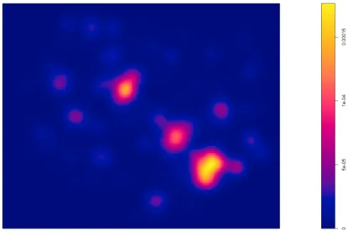
Now the useful data is filtered, it can be analysed. For modelling the spatial part of the spatio-temporal point process, this spatial point process should be chosen in such a way that it represents the spatial point pattern of interest well. But what is the spatial point pattern of interest? For the spatial point process representing a specific class c1a, the spatial point pattern of interest

is the spatial point pattern representing all the emergency calls of this class in Twente for the period on which the model is based, so periodTm. LetSmdenote this spatial point pattern for the classc1a= fire, then figure 2 shows the spatial point pattern of interestSm17.

Analysing the distribution ofSmgives precisely the spatial information for the spatio-temporal point process of interest. A first and quantitative examination of figure 2 indicates already that the distribution of the emergency calls seems aggregated. This will now be formally analysed, following the discussion of section 2.

16_{For a very serious emergency call, firemen of different districts could be summoned. This causes the firemen}

of Twente to go sometimes to an emergency call outside of Twente.

17_{The spatial point pattern plots are made in}_QGIS_{and the data of the borders of the municipalities in Twente}

(25)

[image:25.595.203.397.121.283.2]

Figure 2: Spatial point pattern for the classc1a= fire in the region Twente and in periodTm.

[image:25.595.156.434.354.621.2]