D
EVENTER
J
ULY
2016
R
UBEN
A
KSE
B
ACHELOR
T
HESIS
i
Summary
Modelling Public Transport (PT) is done for many reasons, for example exploring possible new routes for train lines or analyzing commuter flows between two cities. The traditional 4-step model is a way to describe the behavior of a PT system. The last step of the 4-step model describes route-choice for PT travelers.
The route choice algorithm of OmniTRANS, a computer software package to model travel behavior between origins and destinations, is called Zenith. It is based on the frequency-based methodology. Frequency is one of the main inputs for this methodoloy. The choice fractions to board a certain line of a certain path are based on the costs of that path and the frequency of that line. The total average travel time between an origin and destination is based on the average waiting time and the travel time. It appeared that for some path sets the removal of a line led to a lower total average travel time of all paths. This specific model output is counterintuitive and not realistic. In general, there are other disadvantages of the frequency-based methodology such as the average output relative to lines.
The research goals are twofold: firstly there must be determined under which circumstances the specific modelling problem of the total average costs occurs and how this problem has an effect on the modelling output. Secondly, a recommendation should be written based on all advantages and disadvantages of the frequency-based methodology including the outcomes of the analysis of the specific modelling problem.
The theoretical background includes a detailed analysis of the frequency-based algorithm in Zenith and an explanation of the cause of the modelling problem. The literature research discusses other assigning methodologies, such as the scheduled-based methodoloy. This methodology takes into account explicitly all travel times and waiting times.
The methodology to analyze the specific modelling problem consists of two parts. The first part is a sensitivity analysis of how different combinations of input parameters (frequency, travel time) lead to the occurrence of the modelling problem. The second part consists of an analysis of the modelling problem in a large network in OmniTRANS, since it is not known to what extent the modelling problem occurs in practice. This enables to link the theoretical framework of the sensitivity analysis with the practical modelling world. Based on the literature search and the findings of the above-stated first parts, a recommendation is written concerning the frequency-based methodology.
The sensitiviy analysis makes clear that the modelling problem only occurs for low travel-times.
Moreover, only small differences in travel time lead to the modelling problem. In the large case network it appears that the modelling problem occurs quite often (6 % of the stop centroid combinations contains the modelling problem). In case of occurrence of the modelling problem, it appears that the problem severity is low since the difference in travel time (situation with or without a certain line) is small . In general, the theoretical framework matches the outcomes of the large case network.
The recommendation concludes that fixing the specific modelling problem of the total average costs is not that difficult, since the severity is low. But since the frequency-based methodology shows
fundamental modelling problems concerning average modelling output, it is recommended to exploit the possibilites of a new dynamic assignment algorithm in OmniTRANS such as the scheduled-based
methodology. The transit modelling world increasingly needs dynamic models to tackle capacity
ii
Preface
This report is the result of three months of bachelor research for my bachelor graduation thesis. This thesis is the last part of my bachelor, and when successfully completing it I obtain my Bachelor’s degree in Civil Engineering and Management at the University of Twente, Enschede.
This bachelor thesis research has been carried out at DAT.Mobility which is part of Goudappel Coffeng, the largest private mobility consultant of the Netherlands. I have been supervised on a daily basis by Luuk Brederode who is consultant at DAT.Mobility, and by Ties Brands who is consultant at the Public
Transport Department of Goudappel Coffeng. I would like to thank them both for the support on the technical script part of my research as well as for the theoretical background of modelling public transport.
I would also like to thank Tom Thomas, who has supervised me on behalf of the Centre for Transport Studies at the University of Twente. He has given me useful feedback to determine the direction for this research.
iii
Contents
Summary ... i
Preface ... ii
1. Research Context and Problem Definition ... 1
1.1 Modelling Public Transport: Network Definition and 4-step model ... 1
1.2 Modelling Public Transport: determining routes ... 2
1.2 Problem definition: frequency-based methodology ... 3
1.3 Advantages and disadvantages of FB-methodology ... 4
1.4 Motive of research ... 5
1.5 Research goals ... 5
1.6 Research questions ... 5
2. Theoretical Background and Literature ... 7
2.1 Assigning methodology of Zenith in OmniTRANS ... 7
2.2 Cause of the modelling problem in the frequency-based model ... 10
2.3 Literature review of other PT assignment methodologies ... 11
2.4 Summary and conclusion ... 12
3. Methods and models ... 13
3.1 Overview ... 13
3.2 Pre-Analysis of small-case frequency-based model ... 13
3.3 Analysis of large-case frequency-based model ... 15
3.4 Processing the output of the large case network analysis ... 17
4. Results and Discussion ... 19
4.1 Pre-Analysis of small-case frequency-based model ... 19
4.2 Analysis of large-case frequency-based model ... 22
iv
5. Conclusion and Recommendation ... 26
5.1 Conclusion ... 26
5.2 Recommendation ... 27
5.3 Further research possibilities ... 28
6. References ... 29
Appendices ... 30
Appendix A: Selection of stops and centroids in Rotterdam network ... 30
Appendix B: Resulting graphs of pre-analysis ... 32
1
1. Research Context and Problem Definition
Firstly, the research context will be explained. Secondly, the problem definition of this research will be presented. The research context and problem definition together lead to a definition of research goals. The research goals can be translated to research questions.
1.1 Modelling Public Transport: Network Definition and 4-step model
Modelling Public Transport (PT) is done for many reasons, for example exploring possible new routes for train lines or analyzing commuter flows between two cities. The traditional 4-step model is a way to describe the behavior of a PT system (Ortúzar & Willumsen, 2001). This 4-step model is applied to a network, which is the representation of the real life world of roads, PT lines and stops. Firstly the characteristics of the network will be explained, secondly a more detailed explanation the 4-step model will be given.
A passenger transportation network can be considered as a graph with links and nodes. There exist sets of nodes, links, lines and stops. Special nodes are the ones that are origin and destination nodes. From now on these are called centroids. Centroids represent an aggregate number of travelers for a specific time period, in for example a neighborhood. For every centroid the traveler demand is calculated for both origin and destination. All the demands of each centroid are stored in an Origin-Destination Matrix (OD-matrix). For example: the cell (4,5) in an OD-matrix represents the amount of travelers that have centroid 4 as origin and have centroid 5 as destination.
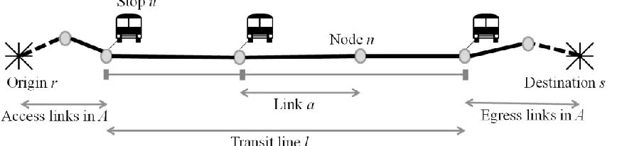
[image:6.612.79.513.547.650.2]In 2007, a new methodology was adopted by DAT.Mobility to describe a multi-modal network in the software package of OmniTRANS (DAT.Mobility, 2016). This methodology is renewed by Brands et al. (2014). The methodology works with legs. A leg is defined as a part of a trip. A trip is defined as going from an origin centroid to a destination centroid. The first leg is from an origin centroid to a stop of PT (e.g. by bike or car). This leg is called the access mode. The second leg is the trip travelled in PT. This leg can have multiple sublegs when a traveller changes services or has to walk for a change of train or bus. The final leg is the leg from the destination stop to the destination centroid. This leg is called the egress mode. An example of such a trip can be seen in Figure 1. In this figure an example is illustrated of a small network. This network contains 8 nodes (of which 2 centroids), 7 links (of which two dashed connectors), 3 stops and 1 PT bus line. The trip displayed in Figure 1 is part of the OD-pair (r,s). In real life, the used network is larger and thus more possible paths are possible between an origin r and a destination s.
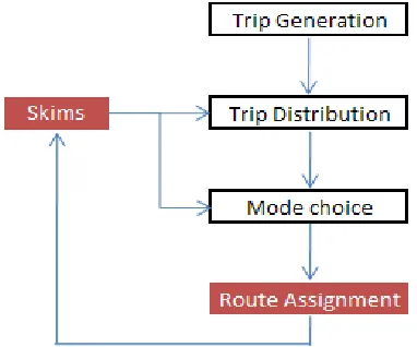
2 In Figure 2, an overview is given of the 4-step model. This model is applied to the above-described
network, to model the behavior of travelers. The first step is Trip Generation: the number of trips is determined for every centroid in a network. This sub model describes trip frequency choice of travelers. The second step is Trip Distribution: in this step all the numbers of trips between centroids are calculated. It describes the destination choice of travelers. The third step is Mode Choice: by what mode is the trip going to take place (e.g. car, train or bike). Trips per OD pair are distributed over modes. Within PT assignment, trip chains are defined. For example, one trip chain can be bike – train – walk. The last step is
Route Assignment: all the trips are assigned on the network. This final step describes route choice. Iterations are done by the use of skims (matrices containing
generalized costs such as cost for travelling for a specific OD pair by a specific mode). Apart from the skim loop in Figure 2, also a loop with time and capacity is running. The model will iterate until an optimum for route assignment is established. This iteration also takes places within the final assignment step, in order to reach user equilibrium on route choice. The skims are used in order to iterate for changing traveler’s mode (mode choice) or destination (trip distribution) due to crowdedness on specific links or transit lines. Not much attention is paid to multi-modal trips in the 4-step model however.
The final assignment step for PT route choice of the 4-step model determines eventually the model output: passenger loads in a network including boarding, alighting and transfer numbers at stops. The most important inputs for the assignment steps are the characteristics of PT lines which are stop type, frequency and in-vehicle travel time.
1.2 Modelling Public Transport: determining routes
The path choice model of OmniTRANS creates possible paths between origins and destinations. Each of these paths have a specific cost which is usually expressed in hours or minutes. When using a value of time, this cost can also be expressed in Euros. This can be useful to calculate the revenue of a newly built transit line, using a social cost and benefits calculation for example (‘MKBA’).
Determining the path set of all paths with corresponding costs between a specific origin and destination is a difficult process. Each path exists of an access leg, transit leg and egress leg as explained in chapter 1.1. The path algorithm works backwards from the destination centroid towards the origin centroid. Only stops that are considered to be realistic are put in the egress stop set. Whether it is realistic is dependent on different things, but the most important thing is the mode. Different modes (e.g. bike, car or walk) can be the egress and access mode.
[image:7.612.75.266.184.343.2]Each stop in the egress stop set is considered to be the final stop in the path. From this stop a tree is built with possible paths towards the origin centroid and its origin access stop. The costs of the transit leg are dependent of in-vehicle travel time, the fare system, the distance covered and possible transfers. The waiting time is not included in these transit costs, and thus calculated separately. By iteration all possible realistic paths between an origin and destination are found, defined for different trip chains.
3 Based on each cost of a possible path, the probability is calculated to board that line which is connected to a specific path. A weighted average cost per stop centroid combination is calculated using the
probability of each path. Secondly, the average waiting time for a specific stop is calculated based on the different frequencies of lines which are part of paths in the path set. The weighted average cost and average waiting time together determine the total average cost to reach a destination from an origin. A more specific and technical description of the path choice model can be seen in chapter 2.1. The average waiting time is calculated using the frequency of each line, and the frequency plays an important role in determining the boarding fractions for each line. Therefore, the above described assignment
methodology is called a frequency-based assignment.
The total average cost of PT per origin and destination can be used to compare PT as main mode with the mode car for example. For an origin and destination, the car costs and PT costs are calculated. Based on these costs iterations are done using skims. Eventually User Equilibrium is established. This is a situation where an equilibrium exists of the traveler choices for mode and route choice. The total average cost of PT is thus the link between the PT sub model and the overall 4-step model which includes all modes. Secondly, the total average cost is used to make analyses of accessibility by different modes. These analyses can be an input for multi-criteria analyses or specific case studies for new transit lines.
1.2 Problem definition: frequency-based methodology
[image:8.612.78.490.525.682.2]A problem which has been encountered with modelling the total average costs has been brought forward by Goudappel Coffeng. This problem is connected with the overall methodology of the frequency-based assignment. The essence of this case is this: adding an extra faster low frequency PT line to an existing slower high frequency line makes the total modelled cost 𝑇𝐶 not lower, but higher. If a line is added, it is expected that the modelled cost will become lower. The problem described by Goudappel Coffeng gives exactly the opposite result which is counterintuitive. This makes the model practically useless since it cannot satisfy its goals such as calculating the amount of extra passengers for a certain od-pair when adding an extra line. The problem can be explained in this way: passengers would experience a lower travel time to go from node 1 to node 2 when an extra line is added, but the Zenith model calculates a higher travel time. An overview of this problem is displayed in Figure 3, including data of each line (f = frequency, tt = in-vehicle travel time). In the next part, the problem will be explained more in depth.
4 The first situation consists of just one line between the two nodes. This line can be characterized as a high-frequency line with a frequency of 6/hour. It takes 20 minutes to go from node 1 to node 2. When calculating the costs to go from o to d according to the methodology described in chapter 1.2, it has been calculated that the total cost (so including waiting time) is 0,417 hrs. (= 24,6 minutes). This methodology assumes that the fare component and transfer component are both zero in the generalized cost formula (1).
The second situation is when a second line is added to the first line. So now the passenger has to choose between two lines: a high frequency line (6/hour) or a low frequency line (1/hour). This low frequency line is faster however; in this case it takes 10 minutes to go from node 1 to node 2. The total travel time in this situation has been composed of the choice fractions of each line multiplied by the travel time, plus the average waiting time at node 1, as described in chapter 1.2. It appears that the total cost in the second situation is 0,437 hrs. (= 26,2 minutes), which is higher than in situation 1.
Goudappel Coffeng knows that this problem occurs in their models since they did some research in specific case studies with high-frequency lines and low-frequency lines. Therefore, it is not known to what extent this problem occurs on a large scale in for example the national train model or the traffic model of Amsterdam. It might be the case that this problem occurs unknowingly quite often, or that it occurs only in very specific cases as studied by Goudappel Coffeng. Therefore, Goudappel Coffeng would like to have more insight on what conditions this modelling problem occurs.
The cause of this problem lies in the path choice models which are described in chapter 1.2. It is unknown what the exact connection is between the most important input of the model (frequency and in-vehicle travel time of each line) and the occurrence of the above-described modelling problem. The classic case of Figure 3 included a high-frequency fast line and a low frequency slow line, but there might be other possible combinations where this situation occurs. Moreover, the modelled problem could also occur at stops where more than two lines halt. In this situation it is even more unclear what the relation is between input and output.
1.3 Advantages and disadvantages of FB-methodology
Using a frequency-based model has advantages in practical sense, but more disadvantages in theoretical sense. The run-time is generally low and therefore the model is easy to handle. In a very complex multimodal PT network, it is easy to insert a frequency. The frequency-based approach produces more aggregate results, which allows only to refer to values relative to lines (Nuzzolo, 2002). Roughly speaking, the frequency approach can be used when a high level of detail is not necessary. In this characteristic lies also the problem with frequency models. One problem is the demand flow varying over the day, or especially over the hour (Cascetta & Copolla, 2016). The OD matrices used in the first two steps of the 4-step model can change: morning-peak matrices and evening-peak matrices do exist. But these matrices are characteristic for just two hours, and within these hours the traffic flow is considered to be static. This is not realistic in commuter flow for example. The supply side of a PT model (input frequencies and thus capacities) is also static during this modelling period. This may lead to underestimation or overestimation of the passenger intensities, since the effect of concentration or dispersion of service capacities is not taken into account with respect to frequency. All in all, the dynamic time component is underexposed in a frequency-based model.
5 handle an average of passengers per hour. Because frequencies are always linked to a unit (per hour, per two hours e.g.), it is difficult to give specific results in a network performance test, such as values of service attributes of single buses or trains. Another effect of average results can be the mismatch between tight transfers, for example from train to bus. When a bus departs only 2 times an hour from a train station, each time 4 minutes after the arrival of a train, the expected waiting time would be 4 minutes in reality. But in the frequency model the average waiting time will be much higher. Therefore, the model does not represent the reality accurate enough. Example of such situations can be seen at the train station of Amersfoort, where two trains come together and have very tight transfer times.
1.4 Motive of research
Apart from the above described theoretical disadvantages, the frequency-based methodology also shows the flaw of the total average cost in a practical sense. All these disadvantages of the frequency-based methodology together are the motivation to research the frequency-based methodology more in-depth, especially the total average cost problem.
1.5 Research goals
This research has several aims which are derived from the research context and problem definition. They are ordered here, including a short explanation with each goal.
1. Gain insight about the circumstances in which the specific problem of the total average costs occurs in practice.
It is not known to what extent the case occurs in practice. It might be the situation that the modelling problem only occurs for very specific od-pairs, travel times or frequencies. More insight in the specific situations of occurrence is needed.
2. Write a recommendation concerning the appropriateness of the frequency-based
methodology for modelling public transport, based on all advantages and disadvantages of the frequency-based methodology.
This research goal puts the research in a larger perspective than just the modelling problem of the total average costs. If it turns out that the occurrence of this modelling problem is quite rare, a specific
solution might not be needed if it is known under which circumstances the modelling problem occurs. But there are still other disadvantages of the frequency-based methodology which are more fundamental. When all disadvantages (modelling problems and their impact) and advantages of the frequency-based methodology are known, a recommendation can be made for Goudappel Coffeng and DAT.Mobility concerning the suitability of the frequency-based methodology.
1.6 Research questions
Based on the described problem context, motive of research and research goals the main question of this research can be defined:
In which cases does the frequency-based Zenith assignment method specifically not give
6 This main question is subdivided in 3 sub questions:
1. Under which circumstances, such as specific od-pairs, frequency and in-vehicle travel time, occurs the problem of the wrong modelled total average costs?
2. How often does the problem of the wrong modelled total average costs occur in practice in a large PT network?
3. To what extent is the frequency-based methodology still the appropriate way to model realistic public transport behavior, based on all advantages and disadvantages including the outcomes of the research concerning the modelling problem of the total average costs?
7
2. Theoretical Background and Literature
The theoretical background is used to deepen the problems of the frequency-based assignment. Firstly, the methodology of the OmniTRANS assigning method Zenith will be explained. This explanation is partly based on the PhD paper of Brands (2015). The methodology already has been described very broadly in chapter 1.2 without formulas. Secondly, by the use of the formulas of Zenith the cause of the total average cost problem can be retrieved. Finally, a literature review has been done in order to know how other PT assigning methodologies work. This helps to contextualize the frequency-based methodology in comparison with other assigning methodologies.
2.1 Assigning methodology of Zenith in OmniTRANS
Let’s assume an individual passenger who travels from an origin o to a destination d by PT. This passenger is part of all the passengers of the OD-pair od. The assigning method determines which PT path the passenger will take. The Zenith methodology consists of 4 steps.
Step 1: Access and Egress Stop Choice
The first step consists of determining the stop choice set, depending on the access and egress mode. For each origin o and destination d centroid, a set of stops is identified from which a PT trip might start or end. It is important to limit the amount of stops in the stop choice set, since including all stops leads to very complex combination of lines and thus to unnecessary computation time. Therefore, for each origin and destination a set with a maximum number of stops is defined, from which a PT trip can begin. This set of stop choice is dependent on the mode by which the access or egress leg will be made, as well as some other criteria such as:
- Distance radius. The radius can be defined differently for both bike and walk, e.g. 4 kilometers. - Type of PT system reached. This factor determines which stop mode is reached, for example bus
or train.
- Type of stop. This factor determines a minimum number of stops of a certain type, for example an intercity station with parking facilities.
- Minimum number of stops. A minimum number of stops has to be in the candidate set.
Candidate sets can be quite different for different access modes such as bicycle, walk or car. Obviously the distance radius plays a big role but also the type of stop can be an important factor. Most of the bus stops cannot be reached by car since parking within a bus stop is not possible. The same methodology of access stop set is applied for the egress stop set. Eventually the first step leads to two stop sets per mode: access stop set and egress stop set for all access and egress modes such as car, walking and bike.
Step 2: Line Choice Model
8 Each link consists of attributes: features that characterize the link. An example of this can be seen in the following Formula (1).
𝐶𝑙𝑖𝑛𝑘 = 𝛼𝑚𝑇𝑙+ 𝛽𝑚𝐾𝑙 + 𝛾𝑚𝑃𝑙 (1)
Where:
𝐶𝑙𝑖𝑛𝑘 Generalized Link costs of a link
𝑇𝑙 On-board Travel time on a link 𝐾𝑙 Fare costs of a link
𝑃𝑙 Penalty for Transfer
𝛼𝑚, 𝛽𝑚 , 𝛾𝑚 Scaling factors dependent of mode
Eventually all generalized costs per link of possible transit lines for the stops are summarized per path. This is done for all stops which are reachable from the candidate set of possible destination stops. These costs are input to calculate the probability to board each of these lines to get from a stop u to a
destination d. Another input for this probability is the frequency of each line. The formula for the probability to board a line is:
𝑝𝑙 =
𝐹𝑙𝑒−𝜆𝐶𝑙
∑𝑥∈𝐿𝐹𝑥𝑒−𝜆𝐶𝑙 (2)
Where:
𝐶𝑙 Generalized costs of a line l
𝐹𝑙 Frequency of line l 𝜆 Zenith scaling factor
𝑝𝑙 Probability of boarding line l
The 𝜆 has been added to control your model output. In theory, if the 𝜆 decreases the boarding fractions 𝑝𝑙 will tend more to the frequency since 𝑒−𝜆𝐶𝑙 will tend more to 1. If 𝜆 increases, 𝑒−𝜆𝐶𝑙 will become larger and thus gets the cost 𝐶𝑙 a larger share in the boarding fraction. This effect can also be seen in the
formula (3) for the combined frequency 𝐶𝐹𝑢𝑚.
A user may consider several lines at one stop, thus the waiting time is calculated by the combined frequency of all lines in the set 𝐿 which have a stop at a certain node (Brands, 2015). The reason to use a combined frequency can be illustrated by this example: consider two lines that have a stop at a certain node. One line is a high frequency line with a large in-vehicle travel time, the other line is a low frequency line with a low in-vehicle travel time. If a passenger arrives at random at the stop, his experienced waiting time is not the average headway of the summarized frequencies, since boarding a slower line gets the passenger earlier at the destination than waiting for the faster line. Therefore a trade-off has been created for the in-vehicle travel time and the frequency in order to create a more realistic experienced waiting time. The combined frequency is dependent on the ratio of the frequency of line l, compared to the summarized frequencies of all lines at this stop u according to Formula 4.
𝐶𝐹𝑢= ∑ 𝐹𝑙
𝑒−𝜆𝐶𝑙𝑢 max
𝑥∈ 𝐿𝑢𝑚𝑒−𝜆𝐶𝑥𝑢
𝑙∈𝐿𝑢𝑚 (3)
Where:
𝐶𝐹𝑢 Combined ‘experienced’ frequency for stop u
9 𝐹𝑙 Frequency of line l 𝐶𝑙𝑢 General cost for line l for stop u
𝜆 Zenith scaling factor
By using this formula, the most attractive line (with the least costs) contributes fully to the combined frequency (factor after 𝐹𝑙 is 1, since the fracture will be equal to 1: nominator and denominator are equal). Less attractive lines contribute to the combined frequency with proportion to the attractiveness of the most attractive line (Brands, 2015, p. 55). For example, two lines have 𝐶𝑙𝑢 of respectively 2 and 4, 𝑒−2= 0.14 and 𝑒−4= 0.018. The maximum is obviously the first value, so the factor after 𝐹𝑙 for this line will be 0.018
0.14 = 0.13. This means that the line with 𝑐𝑙𝑢𝑚 = 4 contributes with a factor of 0.13 of its frequency to the summarized frequency and thus eventually to the combined waiting time.
The combined frequency can be translated to an average waiting time, assuming a random arrival distribution of passengers. This average waiting time has a set maximum of 10 minutes. The average waiting time is an input for the total cost to reach a certain destination from any stop at the network, along with the board probabilities and the in-vehicle travel time. This step is displayed in formula 4:
𝑇𝐶𝑢= min(𝑀𝑊, 𝑊𝑇) + ∑𝑙∈𝐿𝑢𝑚𝑝𝑙𝐶𝑙 (4)
Where:
𝑇𝐶𝑢 Total cost to reach a destination from a stop u
𝑀𝑊 Maximum waiting time at a stop (10 minutes in example)
𝑊𝑇 Waiting time as calculated by the combined frequency
𝑝𝑙 Probability of boarding line l at stop u
𝐶𝑙 Generalized costs of a line l
The above described line choice model can be written down in the following pseudo-code:
Step 1: Determine necessary input
Load network, including link costs 𝐶𝑙𝑖𝑛𝑘
Load all stops
Load all lines, including frequencies 𝐹𝑙 and on-board travel time 𝑇𝑙
Set 𝜆 Set 𝑀𝑊
Step 2: Calculate total average cost For each stop u
For each link
Summarize 𝐶𝑙𝑖𝑛𝑘 to reach a destination d from stop u
End
Calculate line boarding fractions 𝑝𝑙 of each line according to Eq. 2
Calculate 𝐶𝐹𝑢 according to Eq. 3
Calculate Average Waiting Time according to 𝐶𝐹𝑢 and 𝑀𝑊
Calculate Average on-board travel time according to 𝑝𝑙 and 𝑇𝑙
Calculate 𝑇𝐶𝑢 to reach a destination from a certain stop u
End
10 Step 3: including transfers
In step 3 it will be analyzed if adding a walk transfer is decreasing the total cost to reach a destination d
from a stop u. This transfer can occur at one stop where different lines halt, or where a short walk
between two different stops is possible. So for every stop in the network a set of possible transfer stops is created by the use of a walking distance criteria. All of these walking transfers are included at every stop. If the path of a new route (with this extra transfer) has a lower generalized cost, it will be included in the path set of possible routes. This process of searching for new possible paths starting from step 2 will iterate until a maximum number of transfers has been reached. This number can be set in the project set-up.
Step 4: Access Stop Choice
Finally, the access leg is also included in the calculation of the total costs of all possible paths. The chances to board a start stop u, which are in the access stop set, are calculated. These chances are based on the generalized costs per stop u, which are the costs to reach the destination from this stop.
The result of the path choice model is the total average cost, which represents the total cost to reach a destination from an origin. The total average cost is not dependent of the first access leg, since it is calculated from destination centroid to start stop. The final egress leg is thus included.
2.2 Cause of the modelling problem in the frequency-based model
Based on the explanation of the algorithm, it is known how the total average travel time is built up. Now it will be analyzed what causes the modelling problem. To do so, a very simple example will be given of how the total average travel time increases when a line is added.
Consider a line a which has a frequency of 6/hour, and a travel time of 30 minutes. It is the only line in the path set. The average travel time becomes 30 minutes. The experienced frequency is also 6 minutes since there is just one line, thus the average waiting time (assuming random arrival of passengers) is 5 minutes. This means that the total average travel time becomes 35 minutes.
Now, a second line b is added with a frequency of 1/hour and a travel time of 20 minutes. According to formula (2) 60,6% will take line a and 39,4% will take line b (𝜆 = 8). This makes the total travel time based on probabilities 26 minutes. This is 4 minutes lower than the situation where only line a was in the path set. The ‘experienced’ frequency becomes 2,54 according to formula 3. This means that the average waiting time becomes either (1/2,96/2) or 10 minutes according to the first part of formula 4. The
minimum of both is 10 minutes. This is 5 minutes higher than in the situation where only line a was in the path set. The total average travel times becomes thus 10 minutes + 26 minutes = 36 minutes. This is 1 minute more than the situation where only line a was in the path set.
11
2.3 Literature review of other PT assignment methodologies
In this literature review, other assigning methodologies than the frequency-based methodology will be reviewed. This helps to contextualize the research and other methodologies can be an alternative for the frequency-based approach.
In general, two options are available for modelling route choice which is made clear by (TASM, 2014), (Nuzzolo, 2002) and (Poon, 2001). Originally assignment models use the more traditional static
frequency-based approach. Attributes such as waiting time are implicitly considered since the FB model uses averages of waiting time. Recently, a new dynamic path choice approach has been developed which is called the scheduled-based approach.
According to Poon (2001, p.13), the scheduled-based approach refers to ‘services in terms of transit runs, in which the vehicle headway and speed are determined from line schedules’. A more precize description of all the travel times, especially the transfer times can be given. The scheduled-based approach
describes the ‘clock-dependent movement of vehicles within a network as specified in the line schedules’. Therefor the scheduled-based model can be called dynamic. Nuzzolo (2002) adds to this that all the values of service attributes, such as waiting time, can be taken into account in an explicit way.
There are many recommendations in which cases the scheduled-based method should be applied. Generally, a distinction is being made between high-frequency line services and low-frequency line services. High frequency is defined by Nuzzolo (2012) when the average headway is 12-15 minutes, whereas with low-frequency the average headway is 15 minutes or more. The scheduled-based method was initially developped for low frequency systems (Nuzzolo, 2002). When a line has a high frequency, it does not matter whether an user arrives at a stop at 1:00 pm or 1:20 pm. According to Friedrich & Wekeck (2002, p. 3), the schedule-based approach ‘is the appropriate method when precize values for the transfer time, the service frequency and the vehicle loads are expected’. This is especially the case in rural areas or rail networks. Rural areas have low-frequency lines and in the Netherlands the railway system does not have a high-frequency network yet.
A second distinction characteristic between schedule-based and frequency-based is the aim of the model. Frequency-based models are used when an high degree of detail is not needed, and few input data are available (Nuzzolo, 2002). This is especially the case with strategic planning, when only the overall results and expected general movements are taken into account. However, when the aim of a model is about example operative planning, more precize and detailed results are needed.
In a validation research of traffic count data for different modes (High Speed Railway, airplane and car) in Italy, the scheduled-based method and the frequency-based method were compared with each other by Cascetta & Copolla (2016). They found that higher service frequencies (in the range of 2 – 5 trains p/h) were better modelled by the frequency-based method, whereas the scheduled-based model behaves better at lower frequencies (0.33 – 1 train/h). However, in both cases the scheduled-based methodology estimates were overall better than the frequency-based. Also during peak flow, the scheduled-based results were accurate.
12 makes scheduled-based models precious to build and consequently long computation times are
associated with scheduled-based modelling (Friedrich & Wekeck, 2002).
On a larger scale, other choices can be made concerning the assingment methodology. A methdology can be stochastic or deterministic. The deterministic user equilibrium (DUE) assumes that the path choice behavior is deterministic (Cascetta E. , 2001). The supply model (a network) and the demand model (the OD-matrix) is simultaneously applied. Multiple routeing is achieved by the service frequencies or the timetables. The DUE assignment is not capacity dependent, thus it does not take into account crowding effects. Stochastic User Equilibrium (SUE) assumes that there are individual variations in the generalized cost perception (TASM, 2014). This implies that passengers not choose the cheapest option, but the perceived cheapest option. There is an exchange between supply (crowdedness in a network) and the demand (the passengers who choose their path) . This is why SUE assignments can have capacity-constraints per link or line. SUE assignments can also contain more random output since both for passenger and for vehicle departure times random terms can be added. SUE assignments with capacity constrains can be more easily implemented in a scheduled-based assignment, since this methodology is based on the individual runs of each line. The frequency-based methodlogy is not appropriate enough to handle capacity-constraints.
2.4 Summary and conclusion
13
3. Methods and models
The used methodology and models are described. Firstly, an overview of the complete methodology is displayed. This does not only show the different components of the used methodology, but also the consistency between them. Then the individual components are discussed.
3.1 Overview
The overall methodology consists of two parts. The first part is a pre-analysis of a very small frequency-based model case. This analysis will be limited to the case where only two lines connect two centroids. The model that has been used has three input variables, namely: the in-vehicle travel time of each line, the frequency of each line and the Zenith scaling factor. Different scenarios with different combinations of input variables are used as input for two situations: one situation where one line connects the two centroids and the other situation where two lines connect the two centroids. An algorithm determines for both situations the total average costs, which enables to compare both situations. In this way, a
framework can be built to determine in which cases the modelling problem of the total average costs occurs in a theoretical sense. The first part gives answer to sub research question 1.
The second part is a large case analysis for the modelling problem. In order to know to what extent the problem of the total average costs happens on a large scale, an algorithm has been created to analyze PT lines in a network. The aim of this algorithm is to analyze how often, where and on what type of lines the problem occurs in networks. Analyzing the problem on a larger scale also enables to look at more than two lines in one path set between an origin and destination. For example, if there exist 4 paths of four different transit lines between stop u and centroid d, it can be analyzed if removing one of those lines creates a lower total average travel time. If so, this specific stop centroid combination contains the total average cost problem. All stop centroid combinations can be analyzed using the algorithm, whereas the pre-analysis only looks at one theoretical combination.
The large case analysis provides insight for which travel times, stop types, destination types and number of lines in the path set the modelling problem occurs. This enables to link the theoretical framework of the pre-analysis with the practical application of the Zenith assigning methodology. It can be checked whether the found combinations of in-vehicle travel times of the pre-analysis correspond with the found travel times of wrong modelled combinations in the large case analysis. The large case analysis is thus used for both a validation of the pre-analysis and as a source of additional information about the problems of a frequency-based methodology in practice.
3.2 Pre-Analysis of small-case frequency-based model
14 (from 0 to up to the in-vehicle time of line 1). The three in-vehicle travel times for line 1 have been chosen because together they represent enough possible travel times for modes such as bus or train.
The Zenith scaling factor bins are based on commonly used numbers at Goudappel Coffeng for their transit models. The most often used factors are 8 and 10. To analyze also the extreme cases, 6 and 12 have also been added to the possible values of 𝜆.
It is only interesting to analyze the cases where a slow line (line 1) has a high frequency and the fast line (line 2) has low frequency. The lowest frequency possible is 1, so the first combination of frequencies is 2-1. The next frequency combination is 3-2-1. The maximum frequency of line 1 is 6. This value has been chosen because in practice the frequencies are not much higher than 6 for bus or train or tram. The maximum frequency of line 2 is 4. This value has been chosen since a first trial and error run showed that for frequencies higher than 4 the results did not alter anymore.
[image:19.612.78.539.327.385.2]All the input scenarios are displayed in Table 2. The scenarios of Table 2 are run for three scenarios of in-vehicle travel times, which are displayed in Table 1. The results of the pre-analysis are presented in chapter 5.1.
Table 1: Scenarios of in-vehicle travel times
In-vehicle travel time Line 1 [hrs.] In-vehicle travel time Line 2 [hrs.]
0,33 [0 – 0,33]
0,67 [0 – 0,67]
[image:19.612.72.357.427.664.2]1,0 [0 – 1,0]
Table 2: Scenarios pre-analysis part 1 per in-vehicle time of line 1
Zenith scaling factor 𝜆 [1/hr]
Frequency line 1 [1/hr.]
Frequency line 2 [1/hr.]
6
[2..6] 1
[3..6] 2
[4..6] 3
[5..6] 4
8
[2..6] 1
[3..6] 2
[4..6] 3
[5..6] 4
10
[2..6] 1
[3..6] 2
[4..6] 3
[5..6] 4
12
[2..6] 1
[3..6] 2
[4..6] 3
15
3.3 Analysis of large-case frequency-based model
To analyze all stop centroid combinations in a network, an algorithm has been created. The algorithm only looks at paths between stops and centroids, since the route choice algorithm of Zenith is calculated on a stop centroid level as described in chapter 1.2. For each stop centroid combination is thus the total-average travel time calculated, based on different paths with different costs. The total total-average travel time consists of the weighed in-vehicle travel times according to the boarding probability of each path and the average waiting time which is calculated according to the experienced frequency.
The algorithm gets its information from a path engine, which creates paths for a given stop centroid pair. It is possible to create paths with transfers, but processing all this output is too difficult to script.
Therefore, only paths which have direct connections between a stop and a centroid are considered in the algorithm. The only final egress mode is walking. All in all, one possible path that is used for further calculations contains one PT leg (for any mode such as train, bus, metro and tram) and one walk egress leg. The path set of one stop centroid pair can have more than one path, when multiple PT legs exist between a stop and a centroid.
If no direct PT line exists between a pair, the path set for this pair is empty. It can also be the case that there is just one direct PT line between a pair. This case is not interesting, since two lines or more are necessary to reproduce the generalized cost problem. Only the cases where two or more lines are in the path set, are used in further calculations. These calculations reproduce the outcome of the total average costs in the line choice model. Then, one line is deleted from the path set in a systematic way. The total average costs are calculated again. If the total average costs are now lower than in the first situation, the stop-pair is marked and will be put in an output file. If the total average costs are not lower than in the first situation, the next stop centroid pair will be evaluated. It has been chosen not to consider all possible combinations of path sets with deleted lines. In theory, a path set of 4 lines results in 4! = 24
combinations of path sets with deleted lines. Programming this costed too much time. Moreover, if a stop centroid pair is marked when two lines are deleted it will probably also be marked if one line is deleted. This means that looking for more combinations would not be useful. Therefore, it has been chosen to delete only one line from a path set. If there are three in the path set, three situations with one deleted line are compared with the original situation where all lines are input for route choice model. All in all, the algorithm counts four different types of stop centroid combinations:
- No direct path exists between a stop centroid n
- One direct path exists between a stop centroid t
- Two or more direct paths exist between a stop centroid, but the generalized cost problem does not occur q
16 The above described algorithm can be written down in the following pseudo-code:
The used network is a network of the Dutch Randstad, developed by Goudappel Coffeng itself. It contains centroids for the whole Netherlands, but only on a high aggregate level in the Randstad. There are only stops for every mode in the Randstad, outside the Randstad only stops for trains are included. A selection has been made for the stop set and centroid set used in the algorithm. For stops this includes only the agglomeration of Rotterdam including cities such as Spijkenisse, Ridderkerk, Krimpen aan den IJssel and Vlaardingen. For centroids a geographical larger selection has been made, which includes the city of Rotterdam, Den Haag, Gouda, Zoetermeer and Dordrecht. The selections for both the stops and the centroids are displayed in Appendix A. In total there have been selected 1928 stops and 488 centroids. This makes the total possible combinations of stops and centroids 940.864.
This Rotterdam case has been selected since it contains a very diverse range of transit lines, modes and urban densities. All stops that have been selected are in Rotterdam, in order to keep the possible stop centroid combinations lower and thus computation time lower. The centroids are in a larger range. This means that the combinations includes all lines going from Rotterdam to the neighboring destinations. Since it is expected that there are very little direct connections further than the above list of cities for bus or tram no larger selection for centroids has been set, also considering that this would take useless
Step 1: Initialization
Load the network
Load selected list of stops u
Load selected list of centroids d
Set n = 0 Set t = 0 Set q = 0 Set r = 0
Step 2: Create path and do comparison of generalized path cost
For each stop u
For each centroid d
Create path set P in Path Engine
If P is empty
n = n + 1
Elseif P contains 1 path
t = t + 1
Else
Calculate reference generalized path cost Cr
For each line l in P
Delete l
Recalculate generalized path cost C
If C < Cr
r = r + 1
Write output: u, d
Elseif for all lines Cr > C
q = q + 1
End End
End End
17 computation time. A part of Den Haag has been not included in the centroid set, since almost all direct lines coming from Rotterdam end at the train station of Den Haag Centraal or Den Haag HS.
PT lines going from Rotterdam include high frequency lines which go city to city (e.g. Rotterdam to Den Haag) and within cities (e.g. city lines of metro, tram and bus in Rotterdam). There are also low frequency lines in the model from city to city (e.g. intercity train lines between Rotterdam and neighboring cities as Dordrecht) and city to village (e.g. from Rotterdam to small neighboring villages). Also the amount of possible paths is really different. For some stop and centroid which are both in the city of Rotterdam the number of paths can be 6, whereas for other stop centroid combinations which are from Rotterdam to a small village the number of paths can be 2 or 3. The maximum travel time in the selection of stops and centroids is about one hour. This means that the outcomes of the large case model can be compared with the theoretical framework, since the maximum in-vehicle travel time of the pre-analysis also is one hour. All modes possible (including metro and tram) are within the model of Rotterdam. A different mode is not the cause of the occurrence of the modelling problem, since this is only based on frequencies and travel times. But if there exists a correlation between mode, frequencies and travel times this will be reflected in the results of the modelling output. It is interesting to know for DAT.Mobility and Goudappel Coffeng if some modes are more affected by the modelling problem than others on a practical scale.
3.4 Processing the output of the large case network analysis
As described above, the algorithm gives four outputs: n, t, q and r. The route choice model is applied to all cases if one path or more connects a stop and a centroid. This is represented by the output of t, q and r summarized. The line choice model gives not correct results which is represented by the output r. The percentage 𝑝𝑒𝑟𝑐1=
100∗𝑟
(𝑡+𝑞+𝑟) is the first key indicator which is calculated. Since the line choice model strictly can only give ‘wrong’ model output if two lines or more connect a stop and a centroid, the percentage 𝑝𝑒𝑟𝑐2=
100∗𝑟
(𝑞+𝑟) represents the relative occurrence of the modelling problem in the cases of two lines or more connecting a stop and centroid.
To analyze the cases of the modelling problem, firstly a spatial analysis has been done. The modelling output will give insight for which combinations the modelling problem occurs. All these stops and centroids will be analyzed using a spatial map which will display all stops and centroids. This enables to research to what extent a spatial pattern exists between all stop centroid combinations.
Secondly, a detailed analysis has been carried out for all combinations of r. All total average travel times, without the deleted line, have been placed into different classes. All time classes are displayed in Table 3. This has been done for both all rcombinations and the combinations of t, q and r in order to make a comparison between the occurrence percentages specifically for this network.
Table 3: Time classes of detailed analysis
Time Class 1 Time Class 2 Time Class 3 Time Class 4 Time Class 5 Time Class 6
0 – 10 minutes 10 – 20 minutes 20 - 30 minutes 30 – 40 minutes 40 – 50 minutes 50 minutes >
18 frequency is of each deleted line. These numbers also have been ordered in frequency bins. The
difference classes are displayed in Table 4 and the frequency classes are displayed in Table 5.
Table 4: Difference classes of detailed analysis
Difference Class 1 Difference Class 2 Difference Class 3 Difference Class 4 Difference Class 5
0-1 minute 1-2 minutes 2-3 minutes 3-4 minutes 4 minutes >
Table 5: Frequency classes deleted line of detailed analysis
Class 1 Class 2 Class 3 Class 4 Class 5 Class 6 Class 7 Class 8
0,5/hr. 1-1,5 /hr. 2-2,5/hr. 3-3,5/hr. 4-4,5/hr. 5-5,5/hr. 6-6,5/hr. 7/hr. >
Finally, all stop centroids combinations of r and of t, q and r have been placed into four classes of possible paths. The number of paths are the possible transit paths between a stop and centroid before one line has been deleted. It enables to make a comparison between occurrence percentages of the whole network selection and all r combinations. The path classes are displayed in Table 6.
Table 6: Path classes of detailed analysis
Path class 1 Path Class 2 Path Class 3 Path Class 4 Path Class 5 Path Class 6
Nr. of paths = 2 Nr. of paths = 3 Nr. of paths = 4 Nr. of paths = 5 Nr. of paths = 6 Nr. of paths > 7
19
4. Results and Discussion
The results are described in chapter 4. Consequently the results are analyzed and discussed.
4.1 Pre-Analysis of small-case frequency-based model
The first results are the graphs of the in-vehicle travel time combinations, all run for different scenarios of frequency and the Zenith scaling factor. Each unique chart consists of two situations: one with just a high-frequency slow line, and the other situation with a low-high-frequency fast line added. The red line is the result for the travel time of situation 1 where just one slow high-frequency line 1 connects two nodes. Only the travel time of line 1 was input for this line. The black line is the result of situation 2 where the same slow high-frequency line 1 was used, with the fast low frequency line 2 added. Line 2 has different in-vehicle travel times as input (0 – 0,33 hr., 0 – 0,67 hr. and 0 – 1 hr. respectively). Only in-vehicle travel times for line 2 which are lower than the in-vehicle times of line 1, are considered in the charts. Consequently, every chart has been run for different frequency and Zenith scaling factor combinations, as described in the methodology. This leads to three large figures with small sub figures. Each subfigure has a different frequency combination and Zenith Scaling factor. Each large figure has a different in-vehicle travel time for line 1 (0,33 hr., 0,67 hr., 1 hr.). A value in one chart can be interpreted as this, in for example the 0,33 hrs. chart: an in-vehicle time of 0,33 hrs. of line 1 and 0,25 hrs. of line 2 (with 𝜆 = 10 and f1 = 5, f2 = 1)
leads to a total average travel time of 0,43 hr. in situation 1 (red line) and a total average travel time of 0,47 hr. in situation 2 (black line). These numbers can be seen in Figure 4.
In order to clarify the outcomes, graphs have been overlaid. In Figure 5 the overlaying graphs are
[image:24.612.74.335.450.664.2]displayed for an in-vehicle travel time of 0,33 for line 1. In Figure 6 the overlaying graphs are displayed for an in-vehicle travel time of 1,0 for line 1. The left chart displays the first row of each complete graph (𝜆 = 6, frequency differs). The right part displays the last column of each complete graph (frequency = (6,1), 𝜆 differs). The colored numbers correspond with each number of column or row in the complete graph. The complete graphs can be found in Appendix B.
20 The situations where the black line (total travel time situation 2) is higher than the red line (total travel time situation 1) is the situation of the described problem of the generalized costs. Now for each input variable the results will be analyzed and a short conclusion statement will be made.
In-vehicle travel times
In general, it can be seen that a shorter in-vehicle travel time leads to a higher relative occurrence of the situation where the black line is above the red line. This is the case for all situations where the black line is above the red line. Almost half of the total travel times are above the red line for the combination of 0,33 hrs., 𝜆 = 6, f1 = 6 and f2 = 1, whereas this is many times smaller for the same 1,0 hrs. chart.
[image:25.612.61.553.69.467.2]Secondly, relatively small differences of the in-vehicle travel times lead to a situation where the black line above the red line. This effect can already be detected for 0,33 hrs., but it is stronger for higher in-vehicle travel times of line 1. Practically this means that only in a situation of two lines (one high frequency and one low frequency) the generalized cost problem can occur if the difference between the two in-vehicle travel times of each line is small.
Figure 5: Overlapping results for an in-vehicle travel time of 0,33 hrs. for line 1. Left: first row, right: last column
21 Frequency
The frequency has effect on different characteristics in the charts. Firstly, the generalized costs in situation 1 (red line) go down if the frequency of line 1 is higher. The generalized costs in situation 2 (black line) also go down, but the decrease is less than the decrease of the red line. This means that the difference between the red line and black line becomes larger, as the frequency of line 1 is higher.
It can be seen that in all first rows (f1 = 3, f2 = 1) thus for all values of 𝜆 for the three in-vehicle travel times
the black line not underneath the red line gets. This implies that the situation of the generalized cost problem does not occur in this charts for this combination of frequencies.
Zenith scaling factor
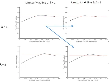
The Zenith scaling factor 𝜆 has a significant effect on the black line. If the 𝜆 increases, the absolute difference between the red line and the black line increases. The relative occurrence of the situation where the black line is above the red line decreases slightly however. The black line graph becomes sharper when the 𝜆 increases and flatter when the 𝜆 decreases. If you look at the effect of the 𝜆 and frequency both together, it can be seen that the black line lies both absolutely higher as the red line and the relative occurrence becomes higher as well. This can be seen in Figure 7. It has already been shown that a higher frequency leads to a higher occurrence of the generalized cost problem. It has also been shown in the theoretical background that an increased 𝜆 leads to a higher proportion of frequency in 𝑝𝑙 and 𝐶𝐹𝑢𝑚. So, a higher 𝜆 leads also to a higher occurrence of the generalized cost problem, when increasing the frequency. The 𝜆 can be seen as a factor that enlarges this process.
[image:26.612.74.434.387.657.2]
22 Based on the charts, it can be concluded that the problem of the total average costs especially occurs in situations where a high frequency line (f1 > 4) is added to a low frequency line (f2 = 1), and where the
in-vehicle travel time of line 1 is not that high (< 30 minutes) and the in-in-vehicle travel time of line 2 is in the range of 1 times and 0.5 times the in-vehicle travel time of line 1. An increasing 𝜆 does not necessarily lead to a higher occurrence of the modelling problem, but it increases the difference of the total average cost between the original situation and the new situation where a line has been added.
4.2 Analysis of large-case frequency-based model
The large case model of Rotterdam has given different outputs which will be given in this chapter. Firstly, the numbers for n, t q and r are presented, including the corresponding percentages of 𝑝𝑒𝑟𝑐1 and𝑝𝑒𝑟𝑐2.
Secondly, a spatial analysis of stops and centroids has been carried out. Thirdly, a detailed analysis has been done. The wrong modelled combinations of r have been placed in different classes for total average travel time, difference between two situations, paths and frequency of deleted line.
Key indicators
The key indicators are summed up:
- No direct path exists between a stop centroid n
- One direct path exists between a stop centroid t
- Two or more direct paths exist between a stop centroid, but the generalized cost problem does not occur q
- Two or more direct paths exist between a stop centroid, and the generalized cost problem does occur r
[image:27.612.76.537.451.483.2]The model output is displayed in Table 7:
Table 7: results of key indicators
n t q r Total
940033 1234 506 126 941899
This makes the percentages 𝑝𝑒𝑟𝑐1and𝑝𝑒𝑟𝑐26 % and 19 % respectively. The first expectation was that this numbers would be lower, so the percentages can be marked as relatively high.
Spatial result
The spatial results are displayed in the Appendices. There are 126 combinations where the wrong modelled total average travel time occurs, of which 27 stops are unique and 86 centroids are unique. Appendix B1 displays the top 12 of stops for which the modelling problem occurs. Appendix B2 displays the top 12 of centroids for which the modelling problem occurs. Finally, Appendix B3 displays all paths of the wrong modelled stop centroid combinations, including the stops and centroids. The different types of transit paths have been split into train, bus & tram and metro. Finally, the egress leg is displayed of each path.
23 lines). A specific pattern of paths cannot be discovered, based on the list of top 12 of stops and centroids. It is remarkable however that most of the top 12 of stops have many lines attached with them. This would mean that stops with many lines are more sensible for the modelling problem than stops with just 2 lines. Finally, it is notable that there are no paths to Den Haag, Gouda or Zoetermeer which all are located further away from Rotterdam. It is unclear why all of these cities do not have a stop centroid path with a wrong modelled total average travel time. This will be analyzed in the discussion in Chapter 5.
Detailed analysis: total average time classes
[image:28.612.74.541.276.380.2]All calculated total average costs of the wrong modelled combinations have been put into classes. In order to analyze for which classes the modelling problem occurs relatively more, the total average costs of all combinations (t, q, r) have also been ordered into the classes. This enables to analyze whether some the modelling problem occurs for lower or higher travel times.
Table 8: Results for total average time classes
0 – 10 minutes
10 – 20 minutes
20 – 30 minutes
30 – 40 minutes
40 – 50 minutes
50 minutes >
Combinations
of r 3 36 42 21 13 11 126
Percentage 2,4 % 28,6 % 33,3 % 16,7 % 10,3 % 8,7 % 100 %
Combinations
of t, q, r 31 310 498 422 302 303 1866
Percentage 1,7 % 16,6 % 26,7 % 22,6 % 16,1 % 16,2 % 100 %
Based on the percentages of Table 8, it can be concluded that the modelling problem specifically occurs for smaller travel times (0 – 30 minutes). The occurrence of r combinations is relatively higher for these bins than for all paths in the network of Rotterdam. For higher travel times (30 – 50 > minutes) the modelling problem occurs relatively less. This is as expected, since the theoretical framework also indicated that the modelling problem happens more for low travel times.
Detailed Analysis: time difference classes
Secondly, for all cases of r the time difference has been calculated between the original total average cost and the new total average cost. In total there are more than 126 numbers, since for one stop centroid combination more than one 1 line can be deleted. If there are for example 5 possible paths for one stop centroid combination, and deleting three lines lead to the wrong modelled total average cost problem, there are three differences of total travel times calculated. The number of stop centroid combinations which are wrong modelled just increases with 1.
Table 9: results of time difference classes
0-1 minute 1-2 minutes 2-3 minutes 3-4 minutes 4 minutes >
Amount 159 18 2 11 2 192
Percentage 83,0 % 9,3 % 1,0 % 5,7 % 1,0 % 100 %
24 Detailed Analysis: path classes
All number of paths of the wrong modelled combinations have been put into classes. In order to analyze for which classes the modelling problem occurs relatively more, the total average costs of all
[image:29.612.74.541.441.487.2]combinations of two paths ore more (q, r) have also been ordered into the classes. This enables to analyze whether some the modelling problem occurs for a higher or lower number of paths.
Table 10: results of path classes
2 3 4 5 6 7 >
Amount 54 15 34 13 3 7 126
Percentage 42,9 % 11,9 % 27,0 % 10,3 % 2,4 % 5,6 % 100 %
Amount 346 99 78 60 3 46 632
Percentage 54,7 % 15,7 % 12,3 % 9,4 % 0,5 % 7,3 % 100 %
The result of the path analysis in Table 10 shows that the modelling problem often happens in an absolute way when there are two paths in the path set, but in a relative way it happens more for paths sets with more than 4 paths. The percentages of all r combinations for these bins are higher than the percentage of the r and q combinations combined. It can be concluded that the modelling problem occurs more when there are more than 4 paths between a stop and a destination. This can also be seen when looking at the top 12 of stops for which the modelling problem occurs. These are all busy stops with many paths.
Detailed Analysis: Deleted frequency classes
For all cases of r,the frequency of the deleted line has been calculated. In total there are more than 126 numbers, since for one stop centroid combination more than one 1 line can be deleted.
0,5/hr. 1-1,5 /hr. 2-2,5/hr. 3-3,5/hr. 4-4,5/hr. 5-5,5/hr. 6-6,5/hr. 7/hr. >
Amount 21 50 19 8 34 6 35 19 192
Percentage 10,9 % 26,0 % 9,9 % 4,2 % 17,8 % 3,1 % 18,2 % 9,9 % 100 %
As expected by the theoretical framework, deleting a low frequency line (0,5 – 1,5 /hr.) leads to a higher total average travel time for many combinations. The number of high frequency lines that are deleted are striking. This was not expected, since the modelling problem only occurs for low frequency lines in theory. This result will be looked at in the discussion.
4.3 Discussion
In the pre-analysis only a case of 2 possible paths has been analyzed. This means that the conclusions of the theoretical framework definitely can be used when there are two paths. When there are more than two paths however, the conclusions can be partially extended to the higher path cases.
25 Figure 8 displays all routes which the path engine gives for possible paths between stop 574 and centroid 1808. The green block displays boarding a line and the red block displays alighting a line. The red chain is the transit part and the orange chain is walking. The path with line 2603 in the opposite direction of the destination has been put in the path set, since the walking distance criteria was set rather high (< 2 kilometers). You first go further away and then you walk back towards the original stop. From this stop you walk back to the final destination. This means that for small distances, illogical paths are also in the path set. The illogical path has a large travel time, since walking takes much time. This means that deleting the path from the path set leads to a lower total average travel time. It can be seen that the boarding probability of each path is 0,71 and 0,29 which is in accordance with the cost of each line. The path engine still gives the illogical path in the path set, since the distances are very small. The r
combinations that were found in this way are not interesting, since the path set itself is not realistic. Therefore, these results can be ignored. This means that the theoretical framework still matches with the large case analysis.
The large case analysis has only been done for direct paths without transfer. This means that the percentages found (perc1 and perc2) could be higher. It is not known to what extent the numbers could
have been higher. It seems legit to assume that the number of extra r combinations due to transfers is higher than the reduction of r combinations due to the illogical path sets on small distances. This means that the percentages found are the same or higher when transfers are added in path sets and the high frequency line cases are deleted in path sets.
Only 1800 stop centroid combinations have been found which are connected by a transit path without any transfer. More numbers were expected. If one transit line has 20 stops on average, and 20 centroids close attached per stop, you would expect 400 possible stop centroid combinations for one line. If there are just 20 lines in a network, you would already expect 8000 stop centroid combinations in total. The number found is many times lower. It can be seen that no wrong modelled path has been found between Rotterdam and Den Haag, Gouda or Zoetermeer. The databases were checked, and it turned out that there was not even a direct line between Rotterdam and Den Haag, Gouda or Zoetermeer (t, q). This means that the path engine, which creates all paths between a given stop and centroid, did not its work properly. It is unknown why this bug occurred, but it might have to do with memory problems of the path engine. It can be concluded that the modelling outcome is not different, since the number of total stop centroid combinations is just a smaller sample of what it could be. This means that the percentages (perc1
and perc2) are still correct.