Mathematical Analysis of the Transmission Dynamics of Tuberculosis

(1)

https://www.scirp.org/journal/ajcm ISSN Online: 2161-1211 ISSN Print: 2161-1203

DOI: 10.4236/ajcm.2019.93012 Aug. 30, 2019 158 American Journal of Computational Mathematics

Mathematical Analysis of the Transmission

Dynamics of Tuberculosis

Jannatun Nayeem*, Israt Sultana

Department of Arts and Sciences, Ahsanullah University of Science and Technology, Dhaka, Bangladesh

Abstract

We develop a dynamical model to understand the underlying dynamics of TUBERCULOSIS infection at population level. The model, which integrates the treatment of individuals, the infections of latent and recovery individuals, is rigorously analyzed to acquire insight into its dynamical features. The phenomenon resulted due to the exogenous infection of TUBERCULOSIS disease. The mathematical analysis reveals that the model exhibits a backward bifurcation when TB treatment remains of infected class. It is shown that, in the absence of treatment, the model has a disease-free equilibrium (DEF) which is globally asymptotically stable (GAS) and the associated reproduction threshold is less than unity. Further, the model has a unique endemic equili-brium (EEP), for a special case, whenever the associated reproduction thre-shold quantity exceeds unity. For a special case, the EEP is GAS using the central manifold theorem of Castillo-Chavez.

Keywords

TUBERCULOSIS Model, SIR Model, Equilibria, Stability, Castillo-Chavez Theorem, Disease Dynamics, Disease Endemic Equilibrium

1. Introduction

A differential equation which describes some physical process is often called a mathematical model of the process. Again a differential equation is a mathemat-ical equation that rates some functions of one or more variables with its deriva-tives, differential equation arises whenever a deterministic relation involving some continuously varying quantities and their rates of change in space and time. These equations occupy the place at center stage of both pure and applied mathematics. For the mathematicians, mathematical modeling offers an impor-tant tool in the study of the evolution of diseases such as Tuberculosis, HIV,

How to cite this paper: Nayeem, J. and Sultana, I. (2019) Mathematical Analysis of the Transmission Dynamics of Tuberculo-sis. American Journal of Computational Mathematics, 9, 158-173.

https://doi.org/10.4236/ajcm.2019.93012 Received: July 9, 2019

Accepted: August 27, 2019 Published: August 30, 2019

http://creativecommons.org/licenses/by/4.0/

(2)

DOI:10.4236/ajcm.2019.93012 159 American Journal of Computational Mathematics Hepatitis, Ebola, etc. Various epidemiology models such as SIR, SEIR, SIRS, SEIS, MSEIR, etc. can be built to analyze these types of diseases. Among them the SIR model is widely used in epidemiology and public health to compute number of individuals in each category of the population and to explain the change in the number of people needing medical attention during an epidemic as well as evaluate policies effectively during the endemic Tuberculosis [1]. The susceptible infected removal (SIR) is a system of ordinary differential equation in three dimensions. SIR model is analyzed by building a mathematical theorem which guarantees the existence of a case of Tuberculosis, the disease free equili-brium phase and stage of disease endemic Tuberculosis [2].

Tuberculosis is an infectious disease usually caused by the Mycobacterium tuberculosis (MTB). Tuberculosis is spread through air, just like a cold or flu when people have active TB in their lungs, they are suffering from cough, spit, speak or sneeze. Tuberculosis generally affects the lungs but it can also be other parts of the body like brain and spine. Tuberculosis is contagious, but it is not easy to catch. It has slow intrinsic dynamics, the incubation period and the infectious period spam long term intervals in the order of years on average. Therefore, a ma-thematical model is needed to have a better insight on the dynamics of the dis-ease [3] [4]. Mathematical models are a simplified representation of how an in-fection spreads across a population over time. Most epidemic models are based on dividing the population into a small number of compartments.

(3)

DOI: 10.4236/ajcm.2019.93012 160 American Journal of Computational Mathematics

[15]. In 2012, there was estimation that 450 thousand individuals developed multidrug-resistant TB (MDR-TB) and an estimation of 170 thousand deaths from MDR-TB [13], which is currently a main threat to tuberculosis control programs and community health [16]. Moreover, an estimated 1.3 million died from this disease and 8.6 million people developed TB under treatment. From 2013 to 2015 it has seen that 6.1 million people developed TB where infected rate was 34%. But TB treatment averted 49 million deaths globally between 2000 and 2015 [16]. It has seen that the rate of infected Mycobacterium tuberculosis (MTB) will reduce day by day, influencing on Bacilli Calmette-Guerin (BCG) vaccines which were first used in 1921 medically in USA and some TB treatment therapies. Tuberculosis infection can be transmitted through primary progres-sion after a recent infection, re-activation of a latent infection and re-infection of a previously infected individual [17]. A small proportion of those infected will develop primary disease within several years of their first infection. Those who escape primary disease may eventually re-activate this latent infection decade af-ter an initial transmission event. Lastly, latently infected individual can be re-infected by a process known as exogenous re-infection and develop the dis-ease as a result of this new exposure [18]. However, if a person got the tuberculosis, then it couldn’t only be seen by the main caution of factors which is causing tuberculosis disease, but also the possibility of exogenous re-infection happening. Tuberculosis is a vaccine prevented disease. The current practice in most part of world especially in developed countries is that children aged 12 to 15 months are given a dose of the BCG vaccine. In practice, even vaccinated individual may still be susceptible if vaccination failure occurred or their vaccine induced immunity waned.

Recent years have seen an increasing trend in the representation of mathe-matical models in publications in the epidemiological literature, from specialist journals of medicine, biology and mathematics to the highest impact generalist journals [19], showing the importance of inter disciplinary.

In this paper, we have formulated the transmission dynamics of Tuberculosis in the presence of treatment and investigated its role in the dynamics of the disease.

2. Formulation of Model

Following the classical assumptions, we formulate a deterministic, compact mental, mathematical model to describe the transmission dynamics of measles. The population is homogeneously mixing and reflecting the demography of a typical developing country, as it experiments an exponentially increasing dy-namics. In other to describe the model equations, the total population (N) is di-vided into three classes: Susceptible (X), infected (Y) and Recovered (Z). Here we shall detail the transitions among these four classes as depicted in Figure 1.

The class X of susceptible is increased by birth or immigration at a rate Λ_{. It}

(4)

DOI:10.4236/ajcm.2019.93012 161 American Journal of Computational Mathematics and therapy at a rate r, breakthrough into infected class at a rate β and dimi-nished by natural death at a rate μ. The class Y of infected individuals is gener-ated by breakthrough of individuals at a rate k. The class is decreased by recov-ery from infection at a rate β and diminished by natural death at a rate μ. The model assumes that both recovered exposed individuals and recovered infected individuals become permanently immune to the disease. This generates a class R of individuals who have complete protection against the disease.

The transitions between model classes can now be expressed by the following system of first order differential equations:

The description of Variables of the TB Model is shown in Table 1.

(

)

1 2

d d

X

Y Z X X r Y r Z

t = Λ −β +η −µ + + (1)

(

)

1

d d

Y

Y Z X k Y

t =β +η − (2)

2 d

d

Z

kY k Z

t = − (3)

Since the model monitors human population, all the associated parameters and state variables are non negative t ≥ 0. It is easy to show that the state va-riables of the model remain non-negative for all non-negative initial conditions. Consider the biological feasible region.

(

)

3

, , :

S I R R N

µ

+

 Λ

Ω =_ ∈ → _

 

[image:4.595.207.526.472.741.2]

From the model Equation (1) to (3) it will be shown that the region is positive. The total population of individuals is given by

Table 1. Description of variables of the TB model.

Variables Description

X Susceptible class

Y Latently infected (exposed) class Z Infected class

Λ Recruitment rate into the population

µ Natural death rate d Death rate due to infection β Probability rate of transmission

1

r Treatment rate for exposed class

2

r Treatment rate for infected class

k Infection rate for exposed individuals

1

k Progression rate of exposed class

2

k Progression rate of infected class

(5)

DOI: 10.4236/ajcm.2019.93012 162 American Journal of Computational Mathematics N = + +S I R

3. Analysis of Model

Disease Free Equilibrium (DFE): The equilibrium points of the system can be obtained by equating the rate of changes of zero, given by ε0,

0 X ,Y 0,Z 0

ε

µ

 Λ 

∴ = = = = 

  (4)

The stability of the DFE will be analyzed using the next generation method

[22]. The non-negative matrix F (of the new infection terms) and the non-singular M-matrix V (of the remaining transfer terms) are given, respectively by,

0 0

F

β βη

µ µ

Λ Λ

 

 

= _ _

 

and 1

2 0

k V

k k

 

= ₋ 

 

where, k1= + +r1 µ k k, 2= + +r2 µ d.

The associated reproduction number, denoted by R0, is given by

(

)

1 0

R =ρ FV− ,

where ρ_{denotes the spectral radius (dominant eigenvalue in magnitude) of}

the next generation matrix FV′. It follows that

1 1

1 2 2

1 0

1

k V

k

k k k

−

 

 

=

 

 

(

2

)

1

1 2 0

k k

FV k k

β η

µ

−

Λ +

 

 

∴ _{= } _

 

 

(

2

)

0

1 2

k k

R

k k

β η

µ

Λ +

∴ = (5)

Lemma: The disease free equilibrium ε0 of the model (1), (2) and (3), is

lo-cally asymptotilo-cally stable (LAS) if R0<1 and unstable if R0>1.

The threshold quantity, R0, is the reproduction number for the model. The

epidemiological implication of Lemma 1 is that Tuberculosis spread can be ef-fectively controlled in the community (when R0<1) if the initial sizes of the

populations of the model are in the basin of attraction of the disease free equili-brium ε0.

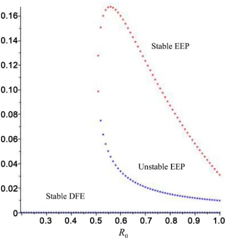
Since we have considered Tuberculosis model in some stages, are shown the backward bifurcation, where the stable DFE co-exists with a stable endemic equilibrium when the associated reproduction threshold (R0) is less than unity,

it is instructive to determine whether or not the model also exhibits this dynam-ical feature. This is investigated below.

(6)

DOI:10.4236/ajcm.2019.93012 163 American Journal of Computational Mathematics 0 1

R = if the inequality holds.

Proof: The proof of theorem, which is based on the use of center manifold theory. The backward bifurcation phenomenon of the model is numerically illustrated be-low. It is convenient to let X =x Y1, =x Z2, =x3, so that N= + +x1 x2 x3.

Fur-ther, by introducing the vector notation

(

)

T

1, 2, 3

X = x x x , the model can be

written in the form,

( )

d d

x F x

t = ,

where

(

)

T

1, 2, 3

F= f f f , as follows

(

)

(

)

1

1 2 3 1 1 1 2 2 3

2

2 2 3 1 1 2

3

3 2 2 3

d d d d d d x

f x x x x r x r x

t x

f x x x k x

t x

f kx k x

t

β η µ

β η

= = Λ − + − + +

= = + −

= = −

(6)

where, λ β=

(

Y+ηZ

)

. The jacobian of the system at the DFE

( )

ε0 is given

by,

( )

0 0

0 J k k d β βη µ µ µ β βη ε µ µ µ µ Λ Λ ₋ ₋ ₋      Λ Λ   =_ − − _    − −     

To analyze the dynamics of the model and we compute the eigenvalues of the jacobian of the equations at the disease free equilibrium (DEF). It can be shown that this jacobian has a left eigenvector is given by

(

)

T

1, 2, 3

V = v v v where,

1 0

v =

2 free

v =

and 3 2

2 v v k βη µ Λ =

The right eigenvector is given by,

(

)

T

1, 2, 3

W = w w w

(

2

)

1 2 2

2 k k w w k β η µ Λ + = − 2 free

w = and 2

3 2 kw w k =

Theorem 2: (Castillo-Chavez and Song)

Consider the following general system of ordinary differential equations with a parameter ϕ.

( )

d , d x f x

t = ϕ , :

n

f ℜ ×ℜ → ℜ and f ∈C

(

ℜ ×ℜn

)

(7)

A1:

( )

0, 0 i

( )

0, 0

x

j

f

A D f

x

_∂ 

= = _ _

∂

  is the linearization matrix of the system (6)

around the equilibrium 0 with ϕ_{evaluated at 0. Zero is a simple eigenvalue of}

A and other eigenvalues of A have negative real parts.

A2: Matrix A has a right eigenvector w and a left eigenvector v (each corres-ponding to the zero eigenvalue).

Let, fk be the kth component of f and

( )

2

, , 1

2 , 1 0, 0 0, 0 n k

k i j

k i j i j

n

k

k i

k i i

f

a v w w

x x

f

b v w

x ϕ = = ∂ = ∂ ∂ ∂ = ∂ ∂

∑

The local dynamics of the system around the equilibrium point 0 is totally de-termined by the sings of a and b. Particularly, a<0,b>0, the system does not

show backward bifurcation at R0=1. In these cases, 0<ϕ1, 0 becomes

un-stable and there exists a positive locally asymptotically un-stable equilibrium. Computations of a and b:

( )

(

)

2

2 1 2 3

, , 1

0, 0 0

n

k k i j

k i j i j

f

a v w w v w w w

x x β η

=

∂

= = + <

∂ ∂

∑

(7)

( )

(

)

2

2 3 2

, 1

0, 0 0

n

k k i

k i i

v w w

f

b v w

x π η ϕ µ = + ∂

= = >

∂ ∂

∑

(8)

This result is summarized below.

Theorem 3: The model (1), (2) and (3) exhibit backward bifurcation at

0 1

R = whenever a<0,b>0. It should be noted that, in the absence of

recov-ery exposed stage and infected stage the backward bifurcation co-efficient, a is given in below,

(

)

2 1 3 2 0

a=βv w ηw +w <

since all the model parameters and the eigenvectors w ii

(

=2, 3,

)

and

(

1, 2,

)

i

v i=  are non-negative and 0< <ε 1. Thus, since the inequality does

not hold in this case, the model (1), (2) and (3) will not undergo backward bi-furcation in the absence of recovery exposed stage and infected stage. This result is summarized below.

Lemma: The model (1), (2) and (3) does not undergo backward bifurcation at

0 1

R = in the absence of treatment (r1= =r2 0). If we consider r1 and r2 exist

then the coefficient of a maybe positive and b is also positive.

The backward bifurcation phenomenon of the model is numerically illustrated in below:

(8)

DOI:10.4236/ajcm.2019.93012 165 American Journal of Computational Mathematics

[20], η=0.08, r1=0.85, r2=0.9, k=0.7 [21].

4. Global Stability of DFE of the TB Model

[image:8.595.229.515.142.436.2]

Let,

Figure 1. Backward bifurcation diagram of susceptible class.

[image:8.595.259.484.466.704.2]

(9)

[image:9.595.249.489.70.318.2]

Figure 3. Backward bifurcation diagram for population of Infected class.

Table 2. Data summary of Parameters of the TB Model.

Parameters Values

Λ 2000 [20]

µ 0.02 [20]

d 0.1 [20]

η 0.08 (assumed)

1

r 0.85 (assumed)

2

r 0.9 (assumed)

k 0.7 [21]

(

)

(

) (

)

d

, d

d

, , , 0 0. d

X

H X Z t

Z

G X Z G X

t

=

= = (9)

where,

(

, 0

)

X = X and Z =

(

Y Z,

)

with the components of 1

X∈R denoting the

uninfected population and the components of _Z_∈_R2 denoting the infected population.

The disease free equilibrium is now denoted as,

(

*

)

*

0 , 0, 0 , , 0, 0

E X X

µ

Λ 

= =  

 

Now, d

(

, 0

)

d

X

H X

t = ,

*

[image:9.595.267.480.368.572.2]

(10)

(

_,

)

ˆ

(

_,

) (

_, ˆ _,

)

₀

G X Z =Pz−G X Z G X Z ≥ for

(

X Z,

)

∈ Ω. (10)

where,

(

*

)

, 0

Z

P=D G X is an M-matrix (the off diagonal elements of P are non

negative) and Ω_{is the region where the model makes biological sense. If the}

system (9) satisfies the conditions of (10) then the theorem below holds.

Theorem 4: The fixed point

(

*

)

0 X , 0

ε _{is a globally asymptotically stable}

equilibrium of system (9) provided that R0<1 and the assumptions in (10) are

satisfied. Proof:

From the system (1) and (2) we have,

(

)

1 2

, 0

0

X r Y r Z

H X = Λ −µ + + _

 

(

)

( )

(

)

(

)

( )

(

)

ˆ

, ,

ˆ _, _,

G X Z P Z G X Z

= −

⇒ = − (11)

where,

( )

1

2 0 k P Z k k −   =  ₋   

and

(

)

1

2

, YX ZX k Y

G X Z

kY k Z

β +βη −

 

=  ₋ 

 

Putting values P Z

( )

and G X Z

(

,

)

in (11) no equation and we obtain,

(

)

(

)

(

)

1

2

ˆ _,

ˆ _, ₀

ˆ _,

G X Z G X Z

G X Z

 

 

=_ _=

  (12)

It is clear that _{G X Z}ˆ

(

_,

)

₌₀_{for all}

(

_{X Z}_,

)

_{∈ Ω}_{we also note that matrix P is}

an M-matrix since its off diagonal elements are non-negative.

5. Endemic Equilibrium Point (EEP) of the TB Model

Let,

(

** ** **

)

1 X ,Y ,Z

ε = represents any arbitrary endemic equilibrium of the

Tuberculosis model. Solving the Equations (1)-(3), the model has the following endemic equilibrium points (EEP),

(

)

(

)(

)

{

}

(

)

(

)(

)

{

}

** 0 2 0 ** 0 2 0 ** 0 2 1 1 X R k R Y

R r d k

k R Z

R r d k

µ

µ µ µ

Λ = Λ − = + + + Λ − = + + +

Existence of Endemic Equilibrium Point (EEP): special case

(11)

Let,

(

** ** **

)

1 X ,Y ,Z

ε = represents any arbitrary endemic equilibrium of the

model (1), (2) and (3) with r1= =r2 0. Solving the equations of the system at

steady-stage gives,

(

)

{

}

(

)

** ** ** 0

X y z

Y y z

Z

β η µ

β η

= − + −

= +

=

(13)

The expression for λ_{, defined in (1), (2) and (3) at the endemic steady-state}

is given by

(

)

**

y z

λ =β +η ₍₁₄₎

For mathematical convenience, the expression in (14) is re-written,

(

)

(

)(

)

{

2 0

}

{

(

0

)(

)

}

**

0 2 0 2

1 1

k R k R

R r d k R r d k

η

λ β

µ µ µ µ µ µ

 Λ − Λ − 

= _ + _

+ + + + + +

 

And we get,

(

)

(

)

(

)(

)

{

0 2

}

**

0 2

1

0

R k k

R r d k

β η

λ

µ µ µ

Λ − +

= >

+ + + (15)

The components of the unique endemic equilibrium ε1 can be obtained by

substituting the unique value of λ**_{, given into the expression in (14). Thus, the}

following has been established.

Lemma: The model with recovery rate from exposed stage and infected stage r1= =r2 0 has a unique endemic equilibrium, given by ε1, whenever

**

0 1, 0

R > λ > .

6. Global Stability of EEP by Non-Linear Lynapunov Function

Theorem 5: The unique EEP

{

}

(

)

(

)(

)

{

}

{

(

)(

)

}

** ** ** 1

2 0 0

0 0 2 1 0 2 1

, ,

1 1

, ,

X Y Z

k R k R

R R r d k R r d k

ε

µ µ µ µ µ µ µ

=

 Λ Λ − Λ − 

 

=  ₊ ₊ ₊ ₊ ₊ ₊ 

 

 

of the

model with r1= =r2 0 is globally asymptotically stable (GAS), whenever

0 1

R > . Proof:

Let, r1= =r2 0 and R0>1, so the EEP, ε1 exists. Consider the following

non-linear Lyapunov function,

** ** ** ** ** **

1

** ** **

ln X ln Y ln Z

L X X X Y Y Y a Z Z Z

X Y Z

     

=_ − − _{ }+ − − _+ _ − − _

      (16)

With Lyapunov derivative is given by,

** ** ** **

2

1 X 1 Y X 1 Z

L X Y Z

X Y k Z

(12)

( )

2 ** ** ** ** ** ** ** 2 2 ** ** ** ** ** ** ** ** ** **

2 Y X

L Y X Z X X X

X

Z X X

YX Y kY

X X

Y Z

XY Y X X Z

Y

β

β βη µ µ

βη µ

β µ

βη

β β βη

= + + − − − − + − − − − + +  (17) And

(

)

** ** 2 2 ** ** ** ** ** ** ** ** ** ** 1 X Z

kY k Z

k Z

Y Z Y

X Z X Z X Z X Z

Z

Y Y

βη

βη βη βη βη

  − −     = − − + (18)

Adding (17) and (18) and we get,

** ** ** ** ** ** ** ** ** ** ** ** ** ** ** 2 2 3

X X X X

X X Y

X X

X Y Z X Y Z

X Z

X Y Z X Y Z

µ β βη     = _ − − _+ _ − − _       + _ − − − _  

Since the arithmetic mean exceeds the geometric mean, it follows then that

** ** ** ** ** ** ** ** 2 0 3 0 X X X X

X Y Z X Y Z

X Y Z X Y Z

− − ≤

− − − ≤

(19)

So that L≤0 for R0>1. Hence, L is a Lyapunov function of the system

with r1= =r2 0 on Ω. In other words,

(

)

(

)

** ** **

lim , , , ,

t→∞ X Y Z = X Y Z .

Thus, by the Lyapunov function L and LaSalle’s Invariance Principle every so-lution to the equation in the model, with r1= =r2 0 approaches ε1 as t→ ∞

for R0>1.

7. Numerical Simulation and Discussions

[image:12.595.215.541.74.343.2]

The effect of the TB transmission dynamics is monitored by simulating the model with the parameters from Table 2. In Figure 4, TB transmission decreas-es gradually with the time where R0<1 (with β =0.9, β =0.09, β =0.09).

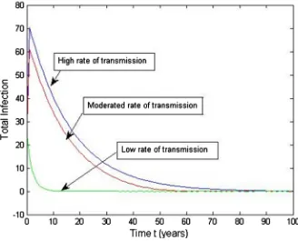
This transmission has to observe as a latent stage with a certain time. In Figure 5, one infected TB patient takes medicine at the rate

(

r1=0.5,r2 =0.5

)

in a

proper time, his infection is decreases rapidly and the infection can be eradicated from the community within very short time. If he takes treatment at the moderate rate

(

r1=0.05,r2=0.05

)

, he cures from the disease gradually day by day with

time. On the other hand, if he takes treatment at the low rate

(

r1=0.005,r2=0.005

)

,

he will be cure from the disease at very slow rate but he gets remove from TB disease at a certain period.

In Figure 6, it is shown that when R0 =0.8544 1< , TB infected person gets

(13)

DOI: 10.4236/ajcm.2019.93012 170 American Journal of Computational Mathematics and TB disease is stable for the value of R0. On the other hand, in Figure 7, it is

shown that when R0=4.7466>1, TB infected person spreads there infection at

a stable stage with a certain time and TB disease is unstable for the value of R0

[image:13.595.208.536.142.407.2]

and the disease can’t eradicate from the community permanantly.

[image:13.595.209.539.412.701.2]

Figure 4. Diagram of TB transmission rate.

(14)

[image:14.595.217.530.57.299.2]

Figure 6. Simulation of the model showing the total number of infected individuals as a

function of time, using the parameters in Table 2 where R0=0.8544<1.

Figure 7. Simulation of the model showing the total number of infected individuals as a

function of time, using the parameters in Table 2 where R0=4.7466>1.

8. Result

We rigorously analyzed (mathematically and numerically) the dynamics of TB in the model. Some mathematical and epidemiological findings of the study are given below:

[image:14.595.216.529.346.597.2]

(15)

DOI: 10.4236/ajcm.2019.93012 172 American Journal of Computational Mathematics stable R0<1 and unstable if R0>1. The model is also globally asymptotically

stable for a special case when r1= =r2 0.

2) When R0 =0.8544 1< , the rate of infected individuals increases and after a

certain time it smoothly decreases.

3) And lastly, the prevalence is very high when R0=4.7466>1.

9. Conclusions

A deterministic model for the transmission dynamics of TB in the population level is designed and rigorously analyzed. Some of the main findings of the study include the following:

1) The model exhibits a phenomenon of backward bifurcation, when DFE is locally asymptotically stable.

2) The model has an EEP which is globally asymptotically stable for special case (i.e. r1= =r2 0).

The model does not undergo backward bifurcation in the absence of treatment stage.

Conflicts of Interest

The authors declare no conflicts of interest regarding the publication of this paper.

References

[1] Kuddus, A., Rahman, A., Talukder, M.R. and Haque, A. (2014) A Modified Sir Model to Study on Physical Behavior among Smallpox Infective Population in Ban-gladesh. American Journal of Mathematics and Statistics, 4, 231-239.

[2] Side, S., Sanusi, W., Aidid, M.K. and Sidjara, S. (2016) Global Stability of SIR and SEIR Model for TB Disease Transmission with Lyapunov Function Method. Asian Journal of Applied Sciences, 9, 87-96.https://doi.org/10.3923/ajaps.2016.87.96

[3] Dago, M.M., Ibrahim, M.O. and Tosin, A.S. (2015) Stability Analysis of a Determi-nistic Mathematical Model for Transmission Dynamics of TB. Proceedings of 32nd The IIER International Conference, Dubai, UAE, 8 August 2015, 42-45.

[4] Adewale, S.O., Podder, C.N. and Gumble, A.B. (2009) Mathematical Analysis of a TB Transmission Model with Dots. Canadian Applied Mathematics Quarterly, 17. [5] Magombedze, G., Garira, W. and Mwenje, E. (2006) Modelling the Human Immune

Response Mechanics to Mycobacterium Tuberculosis Infection in the Lungs. Ma-thematical Biosciences & Engineering, 3, 661-682.

https://doi.org/10.3934/mbe.2006.3.661

[6] Murray, G.J. and Salomon, J.A. (1998) Expanding the WHO Tuberculosis Control Strategy Re-Thinking the Role of Active Case Finding.International Journal of Tu-berculosis and Lung Disease, 2, S9-S15.

[7] Guo, H.B. and Li, M.Y. (2006) Global Stability in a Mathematical Model of Tuber-culosis. Canadian Applied Mathematics Quarterly, 14, 185-197.

(16)

[9] Dubos, R. and Dubos, J. (1952) The White Plogue: Tuberculosis Man and Society. Little and Brown Press, Boston, MA.

[10] Loweell, A., et al. (1996) Tuberculosis. Harvard University Press, Cambridge, MA. [11] Blower, S., Mclean, A.R., Porco, T., Moss, A.R., et al. (1995) The Intrinsic

Trans-mission Dynamics of Tuberculosis Epidemics. Nature Medicine, 1, 815-822.

https://doi.org/10.1038/nm0895-815

[12] WHO (2004) Global TB Control WHO Reports. [13] World Health Organization (2013)

[14] Jakubowiak, W., Bogorods Kaya, E., Borisov, S., Danilova, I. and Kourbatova, E. (2009) Treatment Interruptions and Duration Associated with Default among New Patients with Tuberculosis in Six Regions of Russia. International Journal of Infec-tious Diseases, 13, 362-368.https://doi.org/10.1016/j.ijid.2008.07.015

[15] Feng, Z., Iannelli, M. and Milner, F.A. (2001) A 2 Strain TB Model with Age of In-fection. SIAM Journal on Applied Mathematics, 62, 1634-1656.

https://doi.org/10.1137/S003613990038205X

[16] World Health Organization (2015)

[17] Cohen, T., Colijin, T.C., Finklea, B. and Murray, M. (2007) Exogenous Re-Infection and the Dynamics of TB Epidemics: Local Effects in a Network Model Transmis-sion. Journal of the Royal Society Interface, 4, 523-531.

https://doi.org/10.1098/rsif.2006.0193

[18] Castillo Chavez, C., et al. (2005) A Model of TB with Exogenous Re-Infection.

Theoretical Population Biology, 132, 235-239.

[19] Ferguson, N.M., Cummings, D.A.T., Fraser, C., Cajka, J.C., Cooley, P.C. and Burke, D.S. (2006) Strategies for Mitigating an Influenza Pandemic. Nature, 442, 448-452.

https://doi.org/10.1038/nature04795

[20] Okuonghae, D. and Korobeinikov, A. (2007) Dynamics of Tuberculosis: The Effect of Direct Observation Therapy Strategy (DOTS) in Nigeria. Mathematical Model-ling of Natural Phenomena, 2, 101-113.https://doi.org/10.1051/mmnp:2008013

[21] Sharomi, O., Podder, C.N., Gumel, A.B. and Song, B. (2008) Mathematical Analysis of the Transmission Dynamics of HIV/TB Coinfection in the Presence of Treat-ment. Mathematical Biosciences & Engineering, 5, 145-174.

https://doi.org/10.3934/mbe.2008.5.145

[22] Nayeem, J. and Podder, C.N. (2014) A Mathematical Study on the Vaccination Im-pact on the Disease Dynamics of HBV. IOSR Journal of Mathematics, 10, 26-44.