Voltage Generation by Rotating an
Arbitrary-Shaped Metal Loop around Arbitrary
Axis in the Presence of an Axial Current
Distribution
Constantinos A. Valagiannopoulos
National Technical University of Athens, School of Electrical and Computer Engineering, Division of Electromagnetics, Electrooptics and Electronic Materials, Athens, Greece.
Email: [email protected]
Received March 1st, 2010; revised May 2nd, 2010; accepted May 7th, 2010.
ABSTRACT
A thin metallic wire loop of arbitrary curvature is rotated with respect to an arbitrary axis of its plane. The device is excited by an electric dipole of infinite length and constant current. The resistance of the loop is computed rigorously as function of the position of the source. In this way, the induced voltage along the wire, under any kind of axial excitation, is given in the form of a superposition integral. The measured response is represented for various shapes of the coil, with respect to the time, the rotation angle and the position of the source. These diagrams lead to several technically applicable conclusions which are presented, discussed and justified.
Keywords: Electromagnetic Induction, Arbitrary-Shape Loop, Axial Current Excitation, Superposition Integral
1. Introduction
Electromagnetic (EM) induction is the production of voltage across a conductor situated in a changing mag-netic field or a conductor moving through a stationary magnetic field. The physics that govern the inductive experiments have been mathematically examined in a number of old and elementary studies. The relationship between the various induction laws is summarized in [1] where Cohn advocates that the combined use of both motional and transformer induction assures the validity of the produced results. The Faraday’s disk, the typical DC generator, a cumulative magnet and other inductive structures are thoroughly investigated. Hvozdara also has contributed significantly in analyzing and solving rigor-ously some basic configurations where the EM induction phenomenon appears. For example in [2], the magneto-telluric field for a cylindrical inhomogeneity in a half space with anisotropic surface is evaluated, while in [3] is shown theoretically what effects are generated if one considers the rotation of a spherical Earth in an external inhomogeneous time-variable magnetic field. Moreover, a rudimentary study of induction in a rotating conductor surrounded by a rigid conductor of finite or infinite
ex-tent has been provided in [4]. The analysis is based on integral solutions of the field equations and leads to the conclusion that the induced magnetic fields depend on the relative symmetry of the rotator.
Many solving techniques have been utilized to convert the aforementioned theoretical analyses into practical applications in real-world configurations. For example in [5], a 3-D finite-element general method is presented to treat controlled-source induction problems in heteroge-neous media. It can be used efficiently for EM modeling in mining, groundwater, and environmental geophysics in addition to fundamental studies of EM induction within a heterogeneous environment. Furthermore, many patents and inventions such as [6], exploit inductive phenomena to generate high-voltage power. In particular, the power capability of core-type transformers is in-creased by creating additional magnetomotive force in certain secondary coils without any subsequent power loss. Also in [7], a highly applicable technique is pre-sented which describes finite-difference approximations to the equations of 2-D EM induction that permits dis-crete boundaries to have arbitrary geometrical relation-ships to the nodes.
technical reports, there are numerous recent, state-of- the-art references examining devices and presenting techniques which exploit electromagnetic induction. In [8], a new electromagnetic induction detection mode for Capillary Electrophoresis (CE) and microfluidic chip CE has been presented. Its own optimal operating conditions are determined, and its application in CE and microflu-idic chip CE of inorganic ions is described. A study [9] tests the validity of using electromagnetic induction (EMI) survey data, a new prediction-based sampling strategy and ordinary linear regression modeling to pre-dict spatially variable feedlot surface manure accumula-tion. In addition, a flow injection system incorporating electromagnetic induction heating oxidation for on-line determination of chemical oxygen demand has been proposed [10]. The procedure utilizes induction heating instead of conventional reflux heating, with acidic potas-sium dichromate acting both as an oxidant and as a spec-trometric reagent. Finally, a general-purpose analysis is contained in [11], where the law of induced electromo-tive force is applied to three significant cases: moving bar, Faraday’s and Corbino’s disc.
In this work, we assume a closed metallic wire of arbi-trary shape which is mechanically rotated with respect to an arbitrary axis of its plane, in the presence of an ele-mental source of infinite length and constant current. The parametric equation of the wire curve is extracted through coordinate transformations and the magnetic flux through the loop is evaluated straightforwardly. To this end, we apply the Faraday’s law and an expression for the coil’s resistance is derived. This study examines the voltage induction to the most general case of a single wire loop (shape and rotation axis can be altered at will) which has not been treated rigorously yet. However, the basic novelty of the present analysis is that, due to the linearity of the participating operators, the calculus can be generalized to cover any case of axial excitation. We compute a kind of “Green’s function” ([12]) for the loop impedance, corresponding to a point source excitation. Therefore, the solution for more complex axial currents utilized in industry and technology is given through an integral of that resistance function multiplied by the cur-rent distribution of the source. A set of computer pro-grams has been developed to evaluate the formulas, the induced voltage is represented as function of the time, the rotation angle and the position of the source for vari-ous loop shapes, while the produced graphs are presented and discussed.
2. Problem Statement
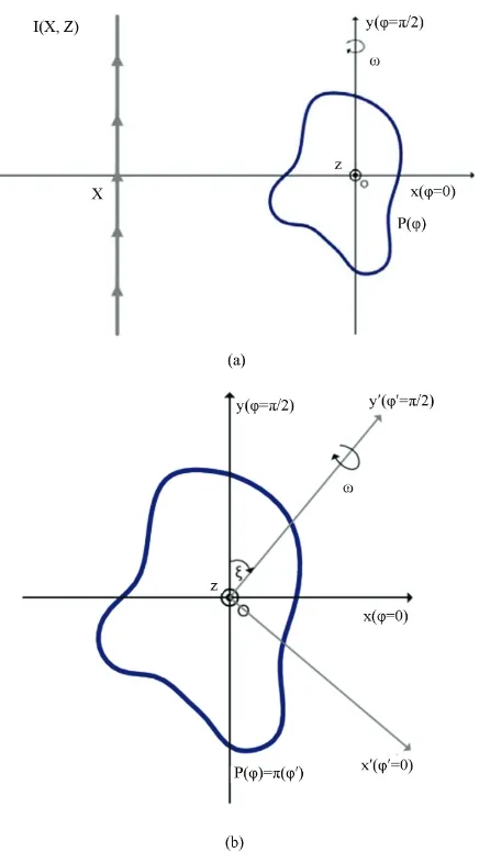
The Cartesian coordinate system ( , , )x y z defined in
Figure 1(a) will be used throughout the analysis. We suppose an infinite axial dipole into vacuum, parallel to
axis, at the position
y (xX z Z, )
)
, flown by a con-stant current (xX z Z,
O
(in Amperes). A wire loop is located around the origin on the ( , )x y plane, and its shape is determined by the radial distance P( )
(polar function) where is the (unprimed) azimuthal angle of our consideration. This closed curve of a perfectly conducting material and infinitesimal thick- ness is rotated periodically around the arbitrary axis
/ 2
with circular frequency , as shown in
Figure 1(b). Consequently, it makes sense just to exam-ine the loop turned by the representative angle t with
[image:2.595.315.533.257.645.2]respect to the aforementioned axis. Initially (t0), the curve lies entirely on the ( , )x y plane.
The purpose of this work is to obtain an expression for the electromotive force induced at the coil, being de-pendent on the time t, the rotation axis and the shape of the loop P( ) . The generated voltage should certainly vary with the position of the primary source
( , )X Z , and thus the derived formula could be used in studying structures with more complicatedly distributed excitation current.
3. Mathematical Formulation
Firstly, we should extract the parametric equation set of the rotated loop when 0 as appeared in Figure 1. The equations will be denoted by {xx( ),φ y y( ),φ
( )}
zz φ and the azimuthal angle will play the role of the parametric variable even when the object does not belong exclusively to
0, 2
φ
( , ) π
x y y
plane. As the closed wire is rotated with respect to axis, the corre-sponding coordinate y( ) will be fixed, independent from the angle t and equal to . The rest two equations are derived by projecting the other edge of length , which is posed at angle
( )sin
P φ φ
( ) coφ sφ
P t, upon
the axes x and Z . Accordingly, one obtains the fol-lowing expressions:
( ) ( ) cos cos
xφ P φ φ ωt, (1)
( ) ( )sin
yφ Pφ φ, (2)
( ) ( ) cos sin
zφ P φ φ ωt. (3) In order to find the parametric equation of the curve when 0
, )
, we use the primed coordinate system
( ,x y z which is received through rotation of the un-primed one by angle with respect to axis Z (de-fined in Figure 1(b)). The polar equation of the loop is now given by ( ) P( ), while the two azi-muthal angles are connected obviously via the relation
p
, }
{ , ,
. Therefore, we take the Formulas (1)-(3) re-placing by and the unprimed variables
x y z by the primed ones { , , , }x y z . In this sense, the parametric set of the primed coordinates with respect to unprimed azimuthal angle (after trivial algebraic manipulations), is written as follows:
( ) ( ) cos( ) cos
xφ Pφ φ ξ ωt (4)
( ) ( )sin( )
yφ P φ φ ξ
(6)
The parametric equations of the arbi loop expressed in the unprimed coor
, (5)
( ) ( ) cos( )sin
zφ Pφ φ ξ ωt
trarily rotated wire dinate system are denoted by
xχ φ( , ),t yψ φ( , ),t zζ φ( , )t
and are determined fr m the transformation relation be ow [13]:( , ) cos sin 0 ( )
χ φt ξ ξ xφ
o l
( , ) sin cos 0 ( )
( , ) 0 0 1 ( )
ψ φt ξ ξ y φ
ζ φt z φ
(7)
An extra time argument has been added to the de-pe
pr
quantities related to the induced volt-ndencies of the parametric equations for better com-ehension.
Once the boundary of the rotating wire is rigorously specified, the field
age can be computed. The magnetic vector potential of a
y-polarized infinite dipole into vacuum at distance D
from its axis is given by [14]:
00 4
( )D μπI
A y ln D
D , (8)
where D0 is the reference distance, 0 is the vacuum
magnet ermeability and y is the itary vector of the y axis. The transverse distance of the representa-tive loop point with azimuthal angle
ic p un
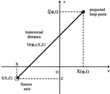
, at an arbitrary time t, from the axis (x X z, Z), is found appar-ently equal to:
2 2
( , , , )
D t X Z (X ( , )t (Z ( , ))t , (9) also shown in Figure 2. It is well-known [15] that the magnetic flux through a closed loop ( )W is defined from the line integral of the magnetic potential on the curve, that is
( )W
Ψ
A Wd . In our case, this formulais particularized [16] to give:
0
2
( , , ) ( , ) ln
π
μ D
Ψ t X Z I X Z
0 ( , , , ) 4
0
( , )
φt X Z
φ
π D ψ φt dφ, (10) where the subscript notation is used for the partial de-rivative of a function. It should be noted that the mag-netic flux is independent from the reference distance D0. According to Faraday’s law, the induced electromotive force is given by the time derivative of magnetic f
/
U
d
Ψ
dt
; therefore, it is sensible to define the lux following auxiliary resistance function by excluding( , )
I X Z from (10):
0
0 2
( , ) ( , , , )
4 ( , , , ) 0
( , , )Z
( , , , ) ln ( , )
φ π
ψ φt
μ Dφt X Z
t φt
π Dφt X Z D
R t X
D φt X Z ψ φt dφ
Figure 2. The transversal distance between the axis of the dipole and a representative point of the rotated loop pro-jected on x-z plane
In this way, the generated voltage on the coil due t o the self-rotation, in the presence of a dipole posed along the axis (xX z Z, ), is given by:
( ) ( , ) ( , , )
U t I X Z R t X Z (12) In case the structure is excited by an axial surface cur-rent distributed according to the law
K X Z
( , )
(meas-ured in /A M), along the line d elec-tromotive force on the wire loop, isth
( )L , the induce
expressed in terms of e following line integral:
( )
( ) ( , ) ( , ,
L
U t
K X Z R t X Z (13)Such an expansion is permissible because the operator
)dL
( )
d
d
dt
W
appliedW
on A to find , is linear. Similarly, if the excitation umeU
is a vol axial current
( , )
J X Z (measured in A m/ 2), across the area ( )S ,
d through the double integral
be-( )
( ) ( , ) ( , , )
S
U t
J X Z R t X Z dS (14)4. Indicative Results
In this se
the voltage is obtaine low:
ction, we examine the produced voltage by ro-tating loops of variable shape and the ef
metrical parameters on it. The described method is wire boundaries possess-ns:
fect of their geo-
plied to two families (A, B) of ing the following polar equatio
2 2
( , , , ) cos n sin n A
P a b n a b , (15)
2 2 2 2
( , , , )
cos sin
B n n
ab
P a b n
a b
, (16)
The arguments
a b,a positive intege
urface
encies
have length dime
argument is r number. For brevity, we chose to excite the structure exclusively t
sources a ng s or volume distributions scribed through (13), (14). The following graphs will ex
re
nsion and the
n
voidi hrough point
de-hibit the depend of the produced voltage U t( )
and the cor sponding RMS value:
2 / 2
0
( ) 2
RMS
U U t dt
(17)A single wire loop is not practically used for voltage generation as clusters of coils are utilized instead. We are more concerned for the qualitative description of the output quantity than measuring t
Volts) of the produced voltage which is extremely small. A
In F
he exact magnitude (in
ccordingly, the so-called “normalized voltage” is rep-resented alternatively which is evaluated by replacing the magnetic permeability of the vacuum 7
0 4 10
2
/
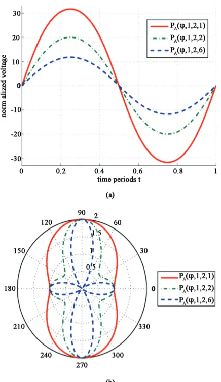
N A in (11), by unity. Each figure below is divided into two subfigures, the first of which is a diagram de-picting the variation of the investigated quantities for various shapes of the loop, while the second is a polar plot of the corresponding wire boundaries.
igure 3(a), we represent the time dependence of the developed normalized voltage for various shapes of loops corresponding to different n parameters of the curve family A with constant a 1 m and b2 m. The observation duration is a single period as from that
cal sym point on the procedure and the results are repeated un-changed. Even though the shape of the wire is arbitrary, the waveforms exhibit typical sinus idal behavior, a fact that can be attributed to the hori d verti -metry of the metallic loop boundary. Also, the amplitude of the oscillation gets greater, as the area of the closed wire increases. This is a natural conclusion because by keeping fixed the rotation frequency and the axis parallel to the dipole, larger loops lead to more significant mag-netic flux variance and implicitly to more substantial output voltage. Therefore, the oscillation amplitude of the investigated quantity is decaying with increasing n
because the occupying area of the loop is greater for 1
n
o nta zo l an
than for n6 as shown in Figure 3(b).
In Figure 4(a), the variation of the RMS value of the induced voltage is depicted as function of the rotation angle for three loop boundaries corresponding different lengths b of the curve family A with constant
m
to
2
t
4(b). a our l at the gl
when b1.5 m. That is because the larger lobes of the curve extend close to the rotation axis in the first case and far from it in he second one as appeared in Figure
ena ll the f obes of the curve are of the same size, which means th obal maximum at
ο
90
the rule according to which, better in-duction results are achieved when the current axis crosses normally the rotation axis of the coil. When
2.5
b m, substantial voltage is produced for a rotation angle close to 45ο, where the response is poor in the
1.5
b m. Needless to say that the graphs are symmetrical with respect to 90ο, due to the canoni-cal shape of the loops.
Wh
reflects
b,
case of
Figu var plots of the
m, ω
re 3. (a) The n ious shapes
bounds. = 100 πrad/se
ormaliz
Pl , D0
Figure 4. (a) The RMS voltage as function of the rotation
In Figure 5(a), we represent the produced voltage as function of the horizontal position of the source
angle for various shapes of the loops; (b) The corresponding polar plots of the bounds. Plot parameters: X = –5 m, Z = 0
m, ω= 100 πrad/sec, D0 = 1 m, I = 1 A, a = 2 m, n = 2
X for three metallic loops with shapes taken from
family B for various parameters ( an the curve
d
n a1 m b
2 m). With increasing X , name
he loop, th m
stantial values. Such u
ect of the field en
e in magnetic flu gh the clo p um point to zer e
the increase is much more rapid
r cases, a result wh h is attributed to t ce between some ts of th
excitation axis when
ly
e induced voltage takes sion is se
er an
s large for
2
when the so
nsible d consequ
sed loo r values. M
3
n
h is loop and th
urce get ore because the
tly, (fro ind than in the e negligi
e sing s
the m a that
ble u-closer to t
eff chang maxim
othe distan lar
a concl gets strong
x throu o) tak
ic poin
X m. Along this region,
ed ion of time for
of the loops. (b) The orresponding polar ot para = 0o, X = -5 m, Z = 0
= 1 m = 1 m, b = 2 m
voltage as funct c meters: ξ , I = 1 A, a
[image:5.595.65.283.283.660.2]Figure 5. (a) The RMS voltage as function of the rotation angle for horizontal positions of the source. (b) The corre-sponding polar plots of the bounds. Plot parameters: ξ= 0ο, Z = 0 m, ω= 100 πrad/sec, D0 = 1 m, I = 1 A, a = 1 m, b = 2 m
th
o In
ese of Figure 4(a). On the other hand, when the pri-mary source gets farther from the rotated wire, its shape plays a rather insignificant role and the differences are mainly attributed to the size of the l op.
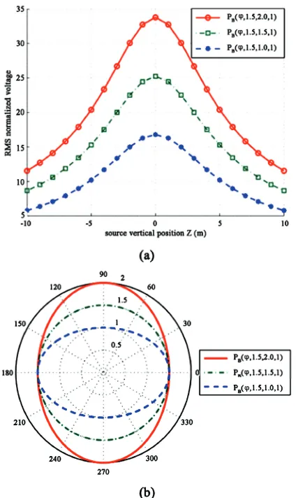
Figure 6(a), the variation of the induced voltage is represented as function of the vertical position of the excitation Z (the source is moving normally to the plane of the sheet) for various loops from curve family B corresponding to different lengths b (with fixed
1.5
a m and n1). In all the three cases the response is maximized for Z 0 which is a al result be-cause the loop is at the closest distance from the excita-tion axis. In addiexcita-tion, the curves are symmetrical with respect to Z 0, due to t t the loops are sym-metric with respect to the rotation axis which is parallel to that of the source ( 0
n r
he fact tha atu
) as shown in Figure 6(b).
Figure 6. (a) The RMS voltage as function of the vertical position of the source for various shapes of the loops. (b) The corresponding polar plots of the bounds. Plot parame-ters: ξ= 0o, X = –5 m, ω= 100 πrad/sec, D
0 = 1 m, I = 1 A, a
= 1.5 m, n = 1
One could point out that the positive effect of the coil’s size on the induced measured quantity is greater when the excitation field is stronger (larger differences be-tween the three curves in the vicinity of Z0). It is al
rc
so remarkable that the induced voltage is exponentially dependent on the distance between the thin closed wire and the sou e current, which is indicated not only by the decrease for large Z in Figure 6(a) but with the in-crease for large X in Figure 5(a) as well.
5. Conclusions
[image:6.595.318.530.97.453.2] [image:6.595.61.285.97.469.2]kind of axial excitation. The time dependence of the measured voltage is of sinusoidal form only if the shape of the loop combined with the rotation axis is symmetric. Additionally, the intuitive guess that the size of the loop, affects positively the inductive action is verified by the numerical results. The distance between the source and the loop is also found to reduce the measured voltage along the coil. As far as the rotation axis is concerned, the most substantial response has been recorded when it is normal to the axis of the dipole current, a result that can have technical applicability.
REFERENCES
[1] G. Cohn, “Electromagnetic Induction,” Electrical Engi-neering, Vol. 1, No. 1, May 1949, pp. 441-447.
[2] M. Hvodara and O. Praus, “Electromagnetic Induction in a Half-Space with a Cylindrical Inhomogeneity,” Studia Ge- ophysica et Geodaetica, Vol. 16, No. 3, September 1972, pp. 240-261.
[3] M. Hvodara and O. Praus, “On Some Effects Connected with Electromagnetic Induction in a Rotating Earth,”
Studia Geophysica et Geodaetica, Vol. 15, No. 2, June 1971, pp. 173-180.
[4] A. Herzenberg and F. Lowes, “Electromagnetic Induction in Rotating Conductors,” Philosophical Transactions of the Royal Society of London, Series A, Mathematical and Physical Sciences, Vol. 249, No. 970, May 1957, pp. 507- 584.
[5] E. Badea, M. Everett, G. Newman and O. Biro, “Finite- Element Analysis of Controlled-Source Electromagnetic Induction Using Coulomb-Gauged Potentials,” Geophysics, Vol. 66, No. 3, 2001, pp. 786-799.
tion on a Feedlot Surface,”
Soil Science Society of America , Vol. 73, No. 6, November 200
[11]
[12]
[13]
[14]
[15]
[6] B. Skillicorn, “Electromagnetic Induction Apparatus for High-Voltage Power Generation,” United States Patent, No. 833436, October 1971.
[7] C. Aprea, J. Booker and J. Smith, “The Forward Problem of Electromagnetic Induction: Accurate Finite-Difference Approximations for Two-Dimensional Discrete Bounda-ries with Arbitrary Geometry,” Geophysical Journal In-ternational, Vol. 129, No. 1, 1996, pp. 29-40.
[8] Z. Chen, O. Lia, C. Liua and X. Yanga, “Electromagnetic Induction Detector with a Vertical Coil for Capillary Elec-trophoresis and Microfluidic Chip,” Sensors and Actuators B: Chemical, Vol. 141, No. 1, August 2009, pp. 130-133. [9] B. Woodbury, S. Lesch, R. Eigenberg, D. Miller and M.
Spiehs, “Electromagnetic Induction Sensor Data to Iden-tify Areas of Manure Accumula
Journal
9, pp. 2068-2077.
[10] S. Han, W. Gan, X. Jiang, H. Zi and Q. Su, “Introduction of Electromagnetic Induction Heating Technique into on-Line Chemical Oxygen Demand Determination,” Interna-tional Journal of Environmental Analytical Chemistry, Vol. 90, No. 2, January 2010, pp. 137-147.
G. Giuliani, “A General Law for Electromagnetic Induc-tion,” Europhysics Letters, Vol. 81, No. 6, February 2008, pp. 1-6.
C. Valagiannopoulos, “Arbitrary Currents on Circular Cylinder with Inhomogeneous Cladding and RCS Opti-mization,” Journal of Electromagnetic Waves and Appli-cations, Vol. 21, No. 5, 2007, pp. 665-680.
L. Hand and J. Finch, “Analytical Mechanics,” Cambridge University Press, Cambridge, 1998, pp. 260-261. M. Sadiku, “Elements of Electromagnetics Oxford Series in Electrical and Computer Engineering,”Oxford Univer-sity Press, Oxford, pp. 284-290.
E. Rothwell and M. Cloud, “Electromagnetics,” CRC Press, Florida, 2003.