https://doi.org/10.1007/s10915-018-0741-7
Numerical Preservation of Velocity Induced Invariant
Regions for Reaction–Diffusion Systems on Evolving
Surfaces
Massimo Frittelli1 ·Anotida Madzvamuse2 · Ivonne Sgura1 ·Chandrasekhar Venkataraman3
Received: 13 December 2017 / Revised: 4 May 2018 / Accepted: 5 May 2018 © The Author(s) 2018
Abstract We propose and analyse a finite element method with mass lumping (LESFEM) for the numerical approximation of reaction–diffusion systems (RDSs) on surfaces inR3that evolve under a given velocity field. A fully-discrete method based on the implicit–explicit (IMEX) Euler time-discretisation is formulated and dilation rates which act as indicators of the surface evolution are introduced. Under the assumption that the mesh preserves the Delaunay regularity under evolution, we prove a sufficient condition, that depends on the dilation rates, for the existence of invariant regions (i) at the spatially discrete level with no restriction on the mesh size and (ii) at the fully-discrete level under a timestep restriction that depends on the kinetics, only. In the specific case of the linear heat equation, we prove a semi-and a fully-discrete maximum principle. For the well-known activator-depleted semi-and Thomas reaction–diffusion models we prove the existence of a family of rectangles in the phase space that are invariant only under specific growth laws. Two numerical examples are provided to computationally demonstrate (i) the discrete maximum principle and optimal convergence for the heat equation on a linearly growing sphere and (ii) the existence of an invariant region for the LESFEM–IMEX Euler discretisation of a RDS on a logistically growing surface.
B
Anotida Madzvamuse [email protected] Massimo Frittelli[email protected] Ivonne Sgura
[email protected] Chandrasekhar Venkataraman [email protected]
1 Dipartimento di Matematica e Fisica “E. De Giorgi”, Università del Salento, via per Arnesano, 73100 Lecce, Italy
2 Department of Mathematics, School of Mathematical and Physical Sciences, University of Sussex, Pevensey III, 5C15, Brighton BN1 9QH, UK
Keywords Evolving surface· Dilation rate·Heat equation·Maximum principle· Reaction–diffusion·Invariant region
1 Introduction
Reaction–diffusion systems (RDSs) are a well-known class of partial differential equations that arise from the mathematical modelling of numerous phenomena taking place on a space-time domain, see for instance [31]. In many applications the spatial domain is a curved surface rather than a flat domain, which may be time-dependent. Among the applications of RDSs on surfaces we mention brain growth [26], cell migration [3], chemotaxis [12], developmental biology [28], electrodeposition [24] and phase field modeling [42]. The growing interest toward PDEs on evolving surfaces has stimulated the development of several numerical methods for such problems, among which we mention (but not limited to) embedding methods [2], kernel methods [18], implicit boundary integral methods [5,35], surface finite element methods (SFEM) [10] and some of their recent variations and extensions [13,16,17,20,23, 40].
An interesting property of some RDSs is the existence ofinvariant regions. An invariant region is a subsetof the phase-space such that, if the initial condition takes values in, then the solution of the RDS takes values inat all times. We recall that, for scalar equations, the well-known notion of maximum principle is equivalent to the invariance of all the regions of the form[0,M], M > 0. For RDSs on a stationary surface, sufficient conditions have been found for a region to be invariant at the continuous level, see [39]. To the best of the authors’ knowledge, the extension of these results to RDSs on evolving surfaces has not been considered in the literature. In this paper we will focus on surfaces that evolve according to a prescribedmaterial velocityfield. More complicated forms of the evolution law are beyond the scope of this manuscript and are a subject of our current studies.
For a numerical method it is interesting to understand if the invariant regions of the continuous problem are preserved under discretisation. In [15,16] we proved that, for RDSs on stationary surfaces, the lumped surface finite element method (LSFEM), combined with an implicit–explicit (IMEX) Euler method, preserves the invariant regions of the continuous problem. The purpose of the present paper is to extend these results to the case of evolving surfaces, in particular (i) we prove a semi- and a fully-discrete maximum principle for the heat equation with a linear source term and (ii) we provide sufficient conditions under which a region is invariant at the semi- and fully-discrete levels when a lumped evolving surface finite element method (LESFEM) and an IMEX Euler timestepping are considered. In particular we quantify the impact of surface evolution (measured through thedilation rate) on the existence of invariant regions and we find that surface growth or contraction respectively fosters or inhibits the invariance of a given region in the phase-space.
the evolving surface, for two well-known RD models in the literature: theactivator-depleted (or Schnakenberg, also known as the Brusselator model) and the Thomas models. Finally, we provide two numerical examples. In the first example we experimentally show that the LESFEM–IMEX Euler method, applied to the heat equation with a linear source term on a linearly growing sphere, exhibits optimal convergence rates in space and time. In the second example we consider the Thomas RDS on an exponentially growing Dupin ring cyclide thereby showing (i) the existence of invariant regions for the fully discretised model and (ii) the violation of this region in the absence of mass lumping.
The present paper is structured as follows. First, in Sect.2we recall (i) the derivation of RDSs on evolving surfaces and (ii) some basic notions about invariant regions and we introduce the notion of dilation rate, which is crucial in our analysis. In Sect.3we introduce the LESFEM for the space discretisation of RDSs on evolving surfaces and we carry out a fully-discrete scheme using the IMEX Euler timestepping. Section4deals with the characterisation of the dilation rate in terms of the material velocity. In particular, we compute exactly the dilation rate for the class of isotropic growth laws. In Sect.5we prove a semi- and a fully-discrete maximum principle for the linear heat equation on evolving surfaces with a linear source term. We prove, in Sect.6, sufficient conditions for the existence of invariant regions for RDSs of arbitrarily many equations on evolving surfaces at the semi- and fully-discrete levels. Section7presents some classes of invariant regions for theactivator-depletedand the Thomas RD models on evolving surfaces, respectively. Numerical examples are presented in Sect.8. Finally, in Sect.9we conclude and discuss our findings with an eye for future extensions of the present work.
2 Reaction–Diffusion Equations on an Evolving Surface
2.1 Preliminaries and Basic Results
Fort ∈ [0,T], letΓ (t)be aC2 orientable surface inR3, represented as the zero-level set
of a signed distance functiond ∈C1([0,T],C2(R3)), i.e.Γ (t)= {x∈R3 |d(x,t)=0}, with∇d(x,t)=0 fort∈ [0,T]andx∈Γ (t). Hence, the outward unit normal vector field onΓ (t)is given by
n(x,t):= ∇d(x,t)
∇d(x,t), t∈ [0,T], x∈Γ (t), (1)
where · denotes the Euclidean norm inR3. Following [10, Section 5], we assume that there exists a mappingG:Γ (0)× [0,T] →R3,G∈C1([0,T],C2(Γ (0))), such that for
allt∈ [0,T],G(Γ (0),t)=Γ (t)andG(·,t)is a diffeomorphism betweenΓ (0)andΓ (t). The space-time surfaceGT is defined byGT :=t∈[0,T]Γ (t)× {t}. The material velocity
v:GT →R3ofΓ (t)is defined by
v(G(x0,t),t)=∂G
∂t (x0,t), ∀x0∈Γ (0), t∈ [0,T]. (2)
Vice-versa, if v˜ ∈ C1([0,T],C2(R3)) is an extension of v, i.e. v˜(G(x0,t),t) =
⎧ ⎨ ⎩
∂G
∂t (x0,t)= ˜v(G(x0,t),t), t∈ [0,T], G(x0,0)=x0.
(3)
Fort∈ [0,T]andδ >0, letUδ(t)be the open neighbourhood ofΓ (t)defined by
Uδ(t):= {(x,t)∈R3× [0,T] : |d(x,t)|< δ}. (4) We recall from [10] the following property.
Lemma 1 (Fermi coordinates) For any t ∈ [0,T]there existsδ > 0 such that for any
x∈Γ (t)there exists a uniquea(x)∈Γ (t)that fulfils
x=a(x)+d(x)n(a(x)), (5) Hence, for t ∈ [0,T], every pointx∈Uδ(t)can be described by d(x)anda(x), which are callednormal coordinatesorFermi coordinatesofx. The functiona(·,t):Uδ(t)→Γ (t)is called thenormal projectionontoΓ (t).
For any sufficiently smoothg:GT →Randg:GT →R3, let∇Γ (t)g,ΔΓ (t)gand∇Γ (t)·g
denote the tangential gradient, the Laplace-Beltrami operator and the tangential divergence ofgonΓ (t), respectively (see [10] for the details). In the following, we will writeΓinstead ofΓ (t)to simplify the notation. Furthermore, let∂•gdenote the material derivative ofg defined by
∂•g:= ∂g˜
∂t +v· ∇ ˜g, (6)
where∇is the standard gradient inR3andg˜is any differentiable extension ofgdefined on a neighborhood ofGT. Definition (6) isintrinsic, i.e. it does not depend on the choice of the extensiong˜(see [11] for further details). Let us recall some basic results from [10].
Lemma 2 (Integration by parts)Ifg :GT →R3 is sufficiently smooth and t ∈ [0,T], it holds that
∂Γ (t)
g·μ=
Γ (t)
∇Γ ·g−
Γ (t)
(g·n)(∇Γ ·n), t∈ [0,T], (7)
whereμ:∂Γ (t)→R3is the outward conormal unit vector on∂Γ (t), i.e. normal to∂Γ (t) and tangent toΓ (t). Specifically, ifgis tangent toΓ, i.e.g·n=0, it holds that
∂Γ (t)
g·μ=
Γ (t)
∇Γ ·g, t∈ [0,T]. (8)
Lemma 3 (Transport formula)For sufficiently smooth g:GT →R, it holds that d
dt
Γ (t) g=
Γ (t)
∂•g+g∇Γ ·v, t∈ [0,T]. (9)
Lemma 4 (Green’s formula on surfaces)For sufficiently smooth f,g :GT →R, it holds that
Γ (t)
∇Γf · ∇Γg= −
Γ (t)
fΔΓg+
∂Γ (t)
Remark 1 (Surfaces without boundary) Lemmas2–4hold on surfaces with or without bound-ary, i.e.∂Γ (t)= ∅or∂Γ (t)= ∅, respectively. Specifically, if∂Γ (t)= ∅, then the boundary integrals in (7), (8) and (10) vanish.
2.2 Derivation of the Reaction–Diffusion Model in Strong Form
Suppose we are givenr∈Nspeciesuk:Γ (t)→R,k=1, . . . ,r, and letqk:Γ (t)→R3, k=1, . . . ,r, be their fluxes tangent toΓ (t). We recall from [1] the derivation of a system ofrequations foru:=(u1, . . . ,ur)that accounts for (i) the diffusion on the surface, (ii) the flux across the boundary (if non-empty) and (iii) the production rates fk(u),k =1, . . . ,r, of the given species. To this end, letR(0)be a portion ofΓ (0)and letR(t)=G(R(0),t) be the portion ofΓ (t)corresponding to the initial portionR(0). Notice thatR(t)is itself an evolving surface, hence formulae (7) through (10) still hold ifΓ (t)is replaced byR(t). We consider a mass balance onR(t)of the form
d dt
R(t)uk = −
∂R(t)qk·μ+
R(t) fk(u), k=1, . . . ,r, t ∈ [0,T]. (11)
Since the fluxesqk,k =1, . . . ,r, are tangent toΓ (t), we can apply the integration-by-parts formula (8) to the first term on the right hand side of (11). Then (11) becomes
d dt
R(t)uk = −
R(t)∇Γ ·qk+
R(t) fk(u), k=1, . . . ,r, t ∈ [0,T]. (12)
By applying the transport formula (9) to the left hand side of (12), we obtain
R(t)
∂•uk+uk∇Γ ·v+ ∇Γ ·qk
=
R(t) fk(u), k=1, . . . ,r, t∈ [0,T], (13)
wherevis the material velocity defined in Sect.2.1. SinceR(t)is an arbitrary portion, we conclude that
∂•uk+uk∇Γ·v+ ∇Γ ·qk= fk(u), k=1, . . . ,r, t∈ [0,T]. (14) We assumeqkcorresponds to a diffusive flux according to Fick’s law as follows:
qk= −dk∇Γuk, ∀k=1, . . . ,r, (15) wheredk,k =1, . . . ,r, are positive diffusivity constants. Inserting (15) into (14), we end up with the reaction–diffusion system of the form
∂•uk+uk∇Γ ·v=dkΔΓuk+ fk(u), k=1, . . . ,r, t∈ [0,T]. (16)
2.3 Invariant Regions and Maximum Principle
In this section we recall basic notions concerning invariant regions for systems of the form (16) and conjecture a sufficient condition under which system (16) possesses an invariant region. To this end, we give the following definitions.
Definition 1 (Dilation rates) Theminimumandmaximum instantaneous dilation ratesare defined by
Hmi n∗ (t):= min
x∈Γ (t)∇Γ ·v(x,t) and H
∗
max(t):= max
respectively. When the minimum and maximum instantaneous dilation rates coincide, we call H∗(t):=Hmi n∗ (t)= Hmax∗ (t)theinstantaneous dilation rate. Theminimumandmaximum global dilation ratesare defined by
μ∗
mi n:= min t∈[0,T]H
∗
mi n(t) and μ∗max := max t∈[0,T]H
∗
max(t), (18)
respectively. When the minimum and maximum global dilation rates coincide, we callμ∗:= μ∗
mi n=μ∗max theglobal dilation rate.
Definition 2 (Invariant regions) For the system (16), a regionin the phase-spaceRr is said to be aninvariant regionif, whenever the initial conditionu0is in, the solutionustays
inas long as it exists and is unique.
We focus our attention on regions⊂Rr of hyper rectangular shape, that is to say of the form
:=
r
k=1
[σk, σk], (19)
whereσk∈R∪ {−∞}andσk∈R∪ {+∞}for allk=1, . . . ,r. For instance, ifσk=0 and σk = +∞for allk =1, . . . ,r, thenis the positive orthant inRr, which means that the solution of the RDS stays positive at all times. Consider the(r−1)-dimensional hyperfaces
k:=∩ {uk=σk}, k:=∩ {uk=σk}, k=1, . . . ,r.
Fork=1, . . . ,r, we define the constants
μ∗k :=
μ∗
mi n ifσk ≥0, μ∗
max ifσk <0, μ
∗
k:=
μ∗
max ifσk≥0, μ∗
mi n ifσk<0,
(20)
whereμ∗mi nandμ∗max are defined in (18).
Next, we conjecture a criterion under which a hyper-rectangle is invariant for system (16). This criterion holds true in the stationary cases (whenμ∗=0): (i) whenΓ is a stationary monodimensional domain inR(see [38]), (ii) whenΓ is a stationaryk-dimensional domain inRk,k∈N(see [6]) and (iii) whenΓis a stationary Riemannian manifold without boundary (see [39]). In the case of isotropically evolving flat domains, the invariance of the positive orthant was studied in [41]. To the best of the author’s knowledge, the case of evolving surfaces has not been studied at the continuous level. Hence, we introduce at the continuous level the following conjecture.
Conjecture 1 Letbe a hyper-rectangle as in(19)in the phase space of(16)and letfbe Lipschitz on. If
fk(u) < μ∗kσk, ∀u∈k∩Rr, ∀k=1, . . . ,r, (21) fk(u) > μ∗
kσk, ∀u∈k∩R
r, ∀k=1, . . . ,r, (22)
thenis an invariant region for(16). In particular, whenσk = +∞andσk= −∞, then k∩Rrand
k∩Rrare respectively empty, and so(21)and(22)are automatically fulfilled, respectively.
We remark that, on stationary domains, some systems are known to possess an invariant region which do not meet the strict inequalities (21)–(22). For instance, for many mass-action laws, the positive orthant is invariant [4,16] even though the flux offis tangent to this region, instead of strictly inward. For the scalar casek=1, the notion of invariant region reduces to the well-known concept ofmaximum principle.
Definition 3 (Maximum principle) Fork=1, the scalar equation (16) fulfils the maximum principle if, for any initial condition, i.e.u(·,0), the solutionufulfils
min
0, min
y∈Γ (0)u(y,0)
≤u(x,t)≤max
0, max
y∈Γ (0)u(y,0)
, (x,t)∈GT. (23)
In particular, if the initial condition is nonnegative,u(y,0)≥0 fory∈Γ (0), the solution fulfils
0≤u(x,t)≤ max
y∈Γ (0)u(y,0), (x,t)∈GT. (24)
Notice that the maximum principle corresponds to the fact that every (monodimensional) region of the form= [σ, σ], withσ≤0,σ≥0, is invariant.
2.4 Derivation of the Variational Formulation
Following [1], we derive the variational formulation of system (16). To this end, for each t ∈ [0,T] we multiply equations (16) by the respective test functions ϕ1, . . . , ϕr ∈
L2([0,T];H1(Γ (t))) with∂•ϕ1, . . . , ∂•ϕr ∈ L2([0,T];H−1(Γ (t))) and integrate over
Γ (t):
Γ (t)(ϕk∂
•u
k+ϕkuk∇Γ·v−ϕkfk(u))=dk
Γ (t)ϕkΔΓuk, (25)
for allk = 1, . . . ,r. For the rigorous definition of the Sobolev spaces H1 andH−1on a manifold see [21], while for the Bochner spacesL2([0,T];B), with Bbeing any Banach space, see [34]. By applying the Green formula (10) to the right hand side of (25) we obtain
Γ (t)(ϕk∂
•u
k+ϕkuk∇Γ·v−ϕkfk(u))+dk
Γ (t)∇Γϕk· ∇Γ
uk=dk
∂Γ (t)ϕk∇Γ
uk·μ,
(26)
for all k = 1, . . . ,r. We assume that either Γ (t) has no boundary, i.e. ∂Γ (t) = ∅, or homogeneous Neumann boundary condition are enforced, i.e.∇Γuk·μ=0 on∂Γ (t), so that the last term in (26) vanishes (see Remark1). Furthermore, by observing that∂•(ϕkuk)= ϕk∂•uk+uk∂•ϕk, (26) becomes
Γ (t)
∂•(ϕkuk)=
Γ (t)
uk∂•ϕk−ϕkuk∇Γ·v+ϕkfk(u)−dk
Γ (t)
∇Γϕk· ∇Γuk,
(27)
for allk=1, . . . ,r. By applying the transport property to the first term on the left hand side of (27), we have
d dt
Γ (t) ϕkuk−
Γ (t)
uk∂•ϕk=
Γ (t)
ϕkfk(u)−dk
Γ (t)
for allk = 1, . . . ,r. Therefore, the variational formulation seeks to find u1, . . . ,ur ∈ L2([0,T];H1(Γ (t)))with∂•u
1, . . . , ∂•ur ∈ L2([0,T];H−1(Γ (t)))such that, for each t∈ [0,T],
d dt
Γ (t)ukϕk−
Γ (t)uk∂
•ϕk+d
k
Γ (t)∇Γuk· ∇Γϕk=
Γ (t) fk(u)ϕk, (29)
for allϕ1, . . . , ϕr ∈L2([0,T];H1(Γ (t)))with∂•ϕ1, . . . , ∂•ϕr ∈L2([0,T];H−1(Γ (t))).
3 Lumped Evolving Surface Finite Element Method
Following the evolving surface finite element method (ESFEM) studied in [1] for the approx-imation of the variational problem (29), we present its lumped counterpart, the lumped evolving surface finite element method (LESFEM).
3.1 Surface Triangulation and Some Definitions
Following [9], givenh >0, calledmeshsize, a triangulationΓh(t)of the evolving surface Γ (t)is defined by
Γh(t)= Z(t)∈Zh(t)
Z(t),
whereZh(t)is a set of evolving triangles, withxi(t),i =1, . . . ,N ∈N, being the overall evolving nodes, such that
– The nodes evolve with the exact material velocity, i.e.x˙i(t)=v(xi(t),t)fort∈ [0,T] andi=1, . . . ,N;
– For allt ∈ [0,T] and for any two distinct triangles Z1(t) and Z2(t) inZh(t), the
intersectionZ1(t)∩Z2(t)is either empty, or a node, or a complete edge;
– For allt∈ [0,T]andZ(t)∈Zh(t),Z(t)⊂Uδ(t), whereUδis as defined in Lemma1; – For allt∈ [0,T], the normal projectiona(·,t):Uδ(t)→Γ (t)defined in Lemma1is a
one-to-one mapping betweenΓh(t)andΓ (t), i.e.a(Γh(t),t)=Γ (t).
We assume that, for eacht ∈ [0,T],Γh(t)meets the Delaunay condition, defined as follows. Letebe an edge ofΓh(t)and letZ1andZ2be the faces ofΓh(t)sharing the edgee. Letα1
andα2be the angles inZ1andZ2opposite toe, respectively. The triangulationΓh(t)is said
to meet the Delaunay condition if, for allt∈ [0,T]and for any edgeeofΓh(t), it holds that
α1+α2≤π, (30)
see for instance [16]. The space-time triangulated surfaceGh,T is defined by
Gh,T :=
t∈[0,T]
Γh(t)× {t}.
SinceΓh(t)is piecewise planar, there exists a time-differentiable mappingGh : Γh(0)×
[0,T] →R3such that, for allt∈ [0,T],Gh(Γh(0),t)=Γh(t)and, for every facetZ∈Zh, Gh(·,t)is a diffeomorphism betweenZ(0)andZ(t).
For a fixed timet∈ [0,T], letVh(t)be the space of piecewise linear functions onΓh(t) defined by
LetVhbe the space of time-dependent, spatially piecewise linear functions defined by
Vh:= {ϕ:Gh,T →R|ϕ(·,t)∈Vh(t)for eacht∈ [0,T]}. (32)
Givent ∈ [0,T]and a functionη ∈ C0(Γh(t)), its linear interpolant Ihη is the unique function inVh(t)such that
Ihη(xi(t))=η(xi(t)), i =1, . . .N.
The discrete material derivative of a sufficiently smooth functionU∈Vhis defined by
∂h•U:= ∂U
∂t +Ih(v)· ∇U, (x,t)∈Gh,T,
wherevis the material velocity. For our purposes, we define the discrete counterpart of the dilation rates introduced in Definition1.
Definition 4 (Discrete dilation rates) Theminimumandmaximum discrete instantaneous dilation ratesare defined by
Hmi n(t):=ess infx∈Γh(t)∇Γh·Ih(v)(x,t),
Hmax(t):=ess supx∈Γh(t)∇Γh ·Ih(v)(x,t), t∈ [0,T], (33) respectively. When the minimum and maximum discrete instantaneous dilation rates coincide, we callH(t):=Hmi n(t)=Hmax(t)thediscrete instantaneous dilation rate. Theminimum andmaximum discrete global dilation ratesare defined by
μmi n:= min
t∈[0,T]Hmi n(t), μmax :=t∈[max0,T]Hmax(t), (34)
respectively. When the minimum and maximum discrete global dilation rates coincide, we callμ:=μmi n=μmaxthediscrete global dilation rate.
For everyi=1, . . . ,N, thei-th Lagrange basis functionχiis the uniqueVh function such that
χi(xj(t),t)=δi j, t∈ [0,T], i,j=1, . . .N, (35) whereδi jis the usual Kronecker symbol. The componentsU1, . . . ,Ur ∈Vhof the spatially discrete solution may be expressed in the Lagrange basis as
Uk(x,t)=
N
i=1
ξk,i(t)χi(x,t), (x,t)∈Gh,T, k=1, . . . ,r. (36)
3.2 Preliminary Results on Triangulated Surfaces
We recall from [9] the following property of the basis functions.
Lemma 5 (Transport property of the basis functions)The basis functionsχi, i=1, . . . ,N , defined in(35)fulfil
∂h•χi=0, i=1, . . . ,N. (37) Hence, for the functions Uk, k=1, . . . ,r defined in(36)it holds that
∂•
hUk(x,t)= N
i=1 ˙
We recall from [10, Lemma 5.6 and Remark 5.7] the following preliminary result.
Lemma 6 (Leibniz formula on triangulated surfaces)For any time-differentiable U,V ∈Vh, it holds that
d dt
Γh(t)
U V =
Γh(t)
∂•U V+
Γh(t)
U∂•V+
Γh(t)
U V∇Γh·Ih(v). (39)
3.3 Lumped Evolving Surface Finite Element Method
The lumped evolving surface finite element method (LESFEM), applied to the variational formulation (29), seeks to findU1, . . . ,Ur ∈Vhsuch that
d dt
Γh(t)
Ih(Ukχi)−
Γh(t)
Uk∂•
hχi+dk
Γh(t)
∇ΓhUk· ∇Γhχi =
Γh(t)
Ih(fk(U)χi), (40)
for allk = 1, . . . ,randi =1, . . . ,N. Thanks to the transport property (37) of the basis functions, formulation (40) is equivalent to: findU1, . . . ,Ur ∈Vhsuch that
d dt
Γh(t)
Ih(Ukχi)+dk
Γh(t)
∇ΓhUk· ∇Γhχi=
Γh(t)
Ih(fk(U)χi), (41)
for allk =1, . . . ,randi=1, . . . ,N. The LESFEM method (41) differs from the evolving surface finite element method (ESFEM) in [1] due to the presence of the interpolant operator on the first and the last terms in (41). By expressingU1, . . . ,Uraccording to (36), the matrix form of (41) is
d
dt(Mξk)+dkAξk=M fk(ξ1, . . . , ξr), k=1, . . . ,r, (42)
whereAandMare the (time-dependent) stiffness and lumped mass matrices defined by
Ai j(t)=
Γh(t)
∇Γhχi· ∇Γhχj, i,j =1, . . . ,N,
Mi j(t)=
Γh(t)
Ih(χiχj)= Γh(t)χi
ifi= j,
0 ifi= j, i,j =1, . . . ,N,
fort∈ [0,T], respectively. Notice that the lumped mass matrixMis diagonal. The Delaunay condition (30) holds if and only if
Ai j(t)≤0, i= j, t∈ [0,T]. (43)
The above fact, together with the structure of the lumped mass matrix implies that, for any s≥0,
(M+s A)−1M(t)≥0, t∈ [0,T]; (44) (M+s A)−1M(t)1=1, t∈ [0,T]. (45)
3.4 Time Discretisation
We are now concerned with the time discretisation of the spatially discrete system (42) arising from the LESFEM. We discretise system (42) by means of the IMEX (IMplicit–EXplicit) Euler method, i.e by treating diffusion implicitly and reaction terms explicitly. To this end, letτ > 0 be a timestep, lettn := nτ for alln =0, . . . ,NT with NT =Tτ, let An and Mn be the stiffness and lumped mass matrices at timetn, respectively, let(ξ1n, . . . , ξrn)be the coefficients of the numerical solution at timetn, and letfnk := fk(ξ1n, . . . , ξnn)for each k =1, . . . ,r. If(ξ10, . . . , ξr0)are the coefficients of the spatially discrete initial datum, the IMEX Euler time discretisation of (42) is
Mn+1ξkn+1−Mnξkn
τ +dkAn+1ξkn+1=Mnfnk, k=1, . . . ,r, n=0, . . . ,NT, (46) or equivalently
ξn+1
k =(Mn+1+τdkAn+1)−1Mn(ξkn+τfnk), k=1, . . . ,r, n=0, . . . ,NT. (47)
4 Characterisation of Surface Growth
The purpose of this section is to characterise surface growth in terms of the material velocity
v, with specific regard to isotropic growth. In fact, the lumped massM(t)and stiffnessA(t) matrices depend onv. In particular:
1. For an arbitrary triangulated surface that evolves with an arbitrary material velocity, we bound the time derivative ddMt of the lumped mass matrix in terms of the constantsμmi n andμmax defined in (34), i.e. in terms of the divergence ∇Γh ·Ih(v) of the discrete material velocity. We will need this result to prove a sufficient condition for the existence of invariant regions for the semi- and fully-discrete schemes;
2. For an arbitrary smooth or triangulated surface that evolves with an arbitrary material velocity, we characterise the velocity flows∇Γ·vand∇Γh·Ih(v)in terms of the mappings GandGhintroduced in Sects.2.1and3.1, respectively;
3. For an arbitrary smooth or triangulated surface that evolvesisotropicallyin space, that is
v(x,t)=S(t)x, (x,t)∈R3× [0,T], (48) whereS : [0,T] →Ris an arbitrary smooth function, we compute exactly∇Γ ·vand
∇Γh ·Ih(v)in terms ofv. This result will yield a fully practical criterion to detect the invariant regions of a given RDS in the case of isotropic surface evolution.
4.1 Bounding the Rate of Change of the Mass Matrix in Terms of the Dilation Rates
In this section we bound the time derivative ddMt ofMin terms of the discrete dilation rates defined in (34). To this end, we prove the following characterisation ofddMt .
Lemma 7 (Transport formula for the lumped mass matrix M)The entries of the lumped mass matrix M fulfil the following property
d dt
Γh(t)
Ih(χiχj)=
Γh(t)
Proof By choosingU=Ih(χiχj)for anyi,j=1, . . . ,NandV=1 in the Leibniz formula (39) we have
d dt
Γh(t)
Ih(χiχj)=
Γh(t)
∂•Ih(χiχ
j)+
Γh(t)
Ih(χiχj)∇Γh·Ih(v). (50)
Now, ifi = j, then Ih(χiχj) = χi, otherwise, ifi = j, Ih(χiχj) = 0. Then, from the transport property (37) we have∂•Ih(χiχj)=0 for alli,j =1, . . . ,N. Equation (50) thus implies the desired result (49).
In some proofs we will need the following corollary of Lemma7.
Corollary 1 (Consequence of the transport formula for the lumped mass matrixM) The diagonal matrixddMt fulfils the estimates
μmi nmii(t)≤dmii
dt (t)≤μmaxmii(t), i =1, . . . ,N, t∈ [0,T], (51) whereμmi nandμmax are defined in(34).
4.2 Characterising Velocity Flows in Terms of the MappingsGandGh
We wish to characterise the continuous and discrete velocity flows∇Γ·vand∇Γh·Ih(v)in terms of the mappingsGandGhintroduced in Sects.2.1and3.1, respectively, for arbitrary smooth or triangulated surfaces that evolve under an arbitrary material velocity. To this end, letΓ (t)be an arbitrary evolving smooth surface and let(A,X)be any local parametrisation ofΓ (0), whereA⊂R2is an open connected set andX:A→Γ (0)is a differentiable map
such that its JacobianJ is full-rank onA. LetBbe a measurable subset ofA. For allt, the portionX(B)ofΓ (0)evolves intoG(X(B),t)⊂Γ (t). By choosing f(x,t)=1 for each (x,t)∈GT in the transport formula (9), we have
d dt
G(X(B),t)1=
G(X(B),t)∇Γ ·v. (52)
Leteiˆ,i=1,2,3, be the standard basis vectors inR3. For(θ,t)∈B× [0,T], letJ(x,t)∈ R2,3be the (spatial) Jacobian of the functionG(X(θ),t)and let
˜
J(θ,t):=
⎡
⎣eˆ1 eˆ2 eˆ3
J(θ,t)
⎤
⎦. (53)
The surface integrals in (52) can be written as integrals on the planar domainBby using the parametrisationG(X(·),t):B→G(X(B),t). Hence, (52) becomes
d dt
B
det(J˜(θ,t))dθ=
B∇Γ ·
v(G(X(θ),t))det(J˜(θ,t))dθ, (54)
where · denotes the Euclidean norm inR3, or equivalently,
B d
dtdet(J˜(θ,t))dθ =
B∇Γ ·
v(G(X(θ),t))det(J˜(θ,t))dθ. (55) Since (55) holds for any measurable subsetBofA, then it holds that
d
By applying the chain rule, (56) is equivalent to
∇Γ ·v(G(X(θ),t))= d
dtlndet(J˜(θ,t)). (57)
Given any triangulated surfaceΓh(t)(which evolves under the discrete velocity fieldIh(v)), we notice that every facetZ(t)∈Zh(t)is smooth and thus parametrisable. For any facet of the initial triangulated surface,Z(0)∈ Zh(0), let(A,X)be a parametrisation of Z(0), as described above. For(θ,t)∈ A× [0,T], letJh(θ,t)∈R2,3be the Jacobian of the function Gh(X(θ),t)and let
˜
Jh(θ,t):=
⎡
⎣eˆ1 eˆ2 eˆ3
Jh(θ,t)
⎤
⎦. (58)
A similar reason as above yields the following discrete counterpart of (57).
∇Γh·Ihv(Gh(X(θ),t))= d
dtlndet(Jh˜(θ,t)). (59)
Relations (57) and (59) are useful in that they (i) express the velocity flow without tangential derivatives and (ii) can be computed exactly whenGandGh are known explicitly, e.g. for the isotropic growth as discussed in the next subsection.
4.3 Computing the Dilation Rates for the Isotropic Growth
In this section we compute the dilation rates defined in (18) and (34), respectively, for arbitrary surfaces that evolve with the material velocity (48). The velocity field (48) corresponds to the specific case of isotropic evolution, see for instance [8,29] for the case of evolving planar domains and [1,32] for the general case. In particular, for suitable choices of the function S(t), the growth law (48) admits some specific cases such as uniform, exponential, logistic and periodic growth, see [1,8,29,32]. From (3), it is easy to show that, with the velocity field (48), eachx0 ∈Γ0evolves to the point
G(x0,t)=exp
t
0
S(τ)dτ
x0, t∈ [0,T], (60)
therefore the evolution induced by an isotropic growth is a time-dependent dilation of the initial surface. The function
φ(t):=exp
t
0
S(τ)dτ
, t∈ [0,T], (61)
that appears in (60) is known as thegrowth function, see for instance [29].
Remark 2 (Properties of isotropic growth) Isotropic growth preserves the angles of triangu-lated surfaces. This has two consequences:
1. ifΓh(0)meets the Delaunay condition, thenΓh(t)retains the Delaunay condition for all t∈ [0,T];
2. ifA(0)andM(0)are the stiffness and the mass matrices att=0, then
A(t)=A(0), M(t)=φ2(t)M(0), t ∈ [0,T]. (62)
In the following result we compute the dilation ratesμmi n,μmax,μ∗mi n andμ∗max on an arbitrary smooth or triangulated surface that evolves with the material velocity (48), in terms ofS(t).
Theorem 1 (Velocity flow on isotropically growing smooth or triangulated surfaces)Let Γ (t) be a smooth surface that evolves with the velocity field (48) and let Γh(t) be the corresponding triangulated surface. Then, the instantaneous dilation rates satisfy
H(t)=2S(t)= H∗(t), t∈ [0,T]. (63) Hence, it follows that
μmi n=μ∗
mi n=2 min
t∈[0,T]S(t), and μmax =μ
∗
max=2 max
t∈[0,T]S(t). (64) Proof LetΓh(t)be an evolving smooth surface and let(A,X),J(θ,t)andJ˜(θ,t)as defined in Sect.4.2. From (60) and (61),J(θ,t)fulfils
J(θ,t)=φ(t)JX(θ), (θ,t)∈A× [0,T], (65)
whereJX :A→R2,3is the Jacobian ofX. It follows that
detJ˜(θ,t) =φ2(t)detJ˜(θ,0), (θ,t)∈ A× [0,T], (66) which implies that
lndetJ˜(θ,t)−lndetJ˜(θ,0)=2 lnφ(t)=2
t
0
S(τ)dτ, (θ,t)∈A×[0,T]. (67)
By differentiating (67), we have
d
dtlndetJ˜(θ,t) =2S(t), (θ,t)∈A× [0,T]. (68) By combining (57), (68) and dropping the parameterised coordinatesθ, we have
∇Γ ·v(x,t)=2S(t), (x,t)∈GT, (69) which proves the first equality in (63). Analogously, we prove the second equality in (63) by using (59). This completes the proof.
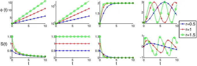
For the uniform, exponential, logistic and periodic growths, the functionsφ(t),S(t)and the dilation ratesμmi n,μ∗mi n,μmax andμ∗max are detailed in Table1, see also [29, Table 1] for the case of evolving planar domains, while the corresponding plots are depicted in Fig.1.
5 Linear Heat Equation and Discrete Maximum Principles
We consider, fork =1, the specific case of linear heat equation on an evolving surfaceΓ (t):
∂•u+u∇Γ ·v=dΔΓu−βu, β∈R, (70) and we prove the semi- and fully-discrete maximum principles for the case whenμmi n+β≥ 0. Equation (70) is a special case of the general system (16) that we are interested in. However, we start with this specific case as (i) it provides more insights on the effect of growth on stability, (ii) we are able to prove a better timestep stability condition and (iii) to make the reader familiar with the demonstrative techniques.
Table 1 Particular types of growth with their respective growth functionsφ(t),S(t)functions and constants
μmi n,μmax,μ∗mi n, andμ∗max
Type of growth Growth functionφ(t) S(t) μmi n=μ∗mi n μmax=μ∗max
Linear r t+1 r
r t+1
2r
r T+1 2r
Exponential exp(r t) r 2r 2r
Logistic Kexp(K r t) K−1+ex p(K r t)
r K(K−1) K−1+exp(K r t)
2r K(K−1)
K−1+exp(K r T) 2r(K−1) Periodic 2−cos(r t) rsin(r t)
2−cos(r t) − 2r√3
3
2r√3 3
The constantr>0 is the growth rate. For the logistic growth,K>1 is thecarrying capacity, i.e. the square root of the ratio between the asymptotical and the initial area of the surface (see [29])
0 5 10
5 10 15
φ (t)
0 5 10
0 0.5 1 1.5 S(t) t
0 5 10
100 105
0 5 10
0 0.5 1 1.5
t
0 5 10
1 1.5 2
0 5 10
0 0.5 1 1.5
t
0 5 10
1 2 3
0 5 10
−1 0 1 t r=0.5 r=1 r=1.5
Fig. 1 Plots of the growth functionsφ(t)(top row) and the correspondingS(t)functions (bottom row) listed in Table1forK=2 andr=0.5,1,1.5. From left to right: linear, exponential, logistic and periodic growth profiles
Theorem 2 (Semi-discrete maximum principle for the linear heat equation (70))If the veloc-ity fieldvfulfils
μmi n+β≥0, (71)
withμmi nas defined in(34), and the triangulationΓh(t)meets the Delaunay condition for all t ∈ [0,T], then the LESFEM solution of(70)fulfils the following discrete maximum principle
min
0, min j=1,...,Nξj(0)
≤ξi(t)≤max
0, max j=1,...,Nξj(0)
, i =1, . . . ,N, t>0.
(72)
Proof From (42), the LESFEM spatial discretisation of (70) is
d
dt(Mξ)+d Aξ = −βMξ. (73)
By applying the chain rule, (73) becomes
Mξ˙+dM
[image:15.439.49.391.217.331.2]By multiplying (74) on the left byM−1, we have
˙
ξ= −d M−1Aξ−M−1dM
dt ξ−βξ. (75)
All we have to prove is that the ODE (75) is dissipative, i.e.−d M−1A|ξ| −M−1 dM
dt |ξ| − β|ξ| ≤ 0. For everyt ∈ [0,T],Mis diagonal with positive diagonal entries and Afulfils (43) from the Delaunay condition. Then, it follows that−d M−1A|ξ| ≤0. Hence, it suffices to prove that−(M−1 ddMt +βI)|ξ| ≤0, that is true provided
M−1dM
dt +βI ≥0. (76)
By using (51), condition (76) is true if
(μmi n+β)I≥0, (77)
which holds true from assumption (71). This completes the proof.
The next theorem shows the same result for the LESFEM–IMEX Euler full-discretisation of (70), under a timestep restriction. This result holds true for the special case of stationary surfaces (see [16, Theorem 2.2]).
Theorem 3 (Fully-discrete maximum principle for the linear heat equation (70))If the veloc-ity fieldvfulfils
μmi n+β≥0, ∀t≥0, (78)
withμmi n as defined in(34), and the triangulationΓh meets the Delaunay condition for all t > 0, then the LESFEM–IMEX Euler solution of(70)fulfils the following minimum-maximum principle
min
0, min j=1,...,Nξ
0
j
≤ξn i ≤max
0, max j=1,...,Nξ
0
j
, i=1, . . . ,N, n=0, . . . ,NT,
(79)
if the timestep satisfies
τβ≤1. (80)
In particular, there is no timestep restriction ifβ≤0.
Proof The full-discretisation (47) of the heat equation (70) can be written as
ξn+1=(Mn+1+τd An+1)−1Mn+1(Mn+1)−1Mn(1−τβ)ξn, n=0, . . . ,NT. (81)
From (44)–(45) we have
(Mn+1+τd An+1)−1Mn+1 ≥0, n=0, . . . ,NT, (82) (Mn+1+τd An+1)−1Mn+11=1, n=0, . . . ,NT. (83) Then scheme (81) fulfils the discrete maximum principle if
Since(Mn+1)−1Mn is diagonal with strictly positive diagonal entries, conditions (84)–(85) are true provided
1−τβ≥0; (86)
(1−τβ)I ≤(Mn)−1Mn+1, n=0, . . . ,NT. (87)
Condition (86) is true under assumption (80). In order to prove (87), we need to estimate Mn+1as a function ofMn. To this end, by applying Gronwall’s lemma to the first inequality in (51), we have
Mn+1≥Mneτμmi n, n=0, . . . ,N
T. (88)
By using (88), condition (87) is true if
1−τβ≤eτμmi n. (89)
Let us now definef(τ):=1−τβandg(τ)=eτμmi n. These functions fulfil f(0)=g(0)=1,
f is linear andgis non-concave for allμmi n∈R. Then
– if f(0) >g(0), then condition (89) is not fulfilled for any sufficiently smallτ. – if f(0)≤g(0), then condition (89) is fulfilled for everyτ >0.
Now, condition f(0)≤g(0)means−β≤μmi n, which is true from assumption (78). This completes the proof.
Remark 3 (Interplay between material velocity and source term) Relation (71) implies that
– domain growth (μmi n>0) can enable the discrete maximum principle even forβ <0; – local domain contraction (μmi n <0) can prevent the discrete maximum principle even
forβ≥0.
This interplay is justified by observing that domain evolution implies a dilution effect, explained as follows. By choosingϕ = 1 in the variational formulation (29) withk = 1 and f1(u)= −βu, we obtain
d dt
Γ (t) u= −β
Γ (t)
u, t∈ [0,T]. (90)
If|Γ (t)|denotes the surface area ofΓ (t)andu(t) := |Γ (1t)|Γ (t)udenotes the mean value ofu, (90) becomes
d
dt(|Γ (t)|u(t))= −β|Γ (t)|u(t), t ∈ [0,T]. (91)
By solving (91) forddtu(t), we obtain
d
dtu(t) = −
β|Γ (t)| + d dt|Γ (t)|
|Γ (t)| u(t), t∈ [0,T]. (92)
By choosingg=1 in the transport formula (9), we have
d
dt|Γ (t)| =
Γ (t)
∇Γ·v≥ |Γ (t)|μmi n∗ , t∈ [0,T]. (93)
By combining (92) and (93) we have
d
dtu(t) ≤ −(β+μ
∗
From (94), the dilution effect arising from surface growth can be interpreted as the dampening or uplifting effect ofμ∗mi nonu(t). The estimate (94) implies thatu(t)is non-increasing if
β+μ∗
mi n≥0, (95)
which is the continuous counterpart of (71). We conclude that condition (71) is consistent with the interpretation of surface growth in terms of dilution effect.
Remark 4 (Interplay between timestep restriction and source term) Relation (80) implies that the timestep restriction needed for guaranteeing the discrete maximum principle is indepen-dent of the material velocity and it only depends on the stiffness parameterβof the source term. In particular, when the source term is nonnegative (i.e. whenβ ≤0), the LESFEM– IMEX Euler fully-discrete scheme unconditionally fulfils the discrete maximum principle.
6 Reaction–Diffusion Systems and Invariant Regions
In this section we prove, for the semi- and full-discretisations of RDSs of the form (16), a criterion to test if a hyper-rectangle in the phase-space is invariant. In the casek=1 of scalar equations, the notion of invariant region collapses to that of minimum-maximum principle, considered in the previous section for the special case of the linear heat equation. We assume that the Delaunay regularity of the mesh is preserved under evolution. Fork=1, . . . ,r, we define the constants
μk:=
μmi n ifσk≥0,
μmax ifσk<0, μk:=
μmax ifσk≥0,
μmi n ifσk<0, (96)
whereμmi n andμmax are the dilation rates defined in (34). In the following theorem we prove that, under similar assumptions of Conjecture1, is an invariant region for the solution obtained from the semi-discrete scheme (42). Hence, the following theorem extends [16, Theorem 3.3] to the case of evolving surfaces.
Theorem 4 (Invariant rectangles for (42)) Let be a hyper-rectangle as in (19) in the phase space of(42), letfbe Lipschitz on. If the triangulationΓh(t)satisfies the Delaunay condition for all t≥0and
fk(U) < μkσk, ∀U∈k∩Rr, ∀k =1, . . . ,r, (97) fk(U) > μkσk, ∀U∈k∩Rr, ∀k =1, . . . ,r, (98) thenis an invariant region for(42).
Proof The semi-discrete method (42) can be written, after applying the chain rule to the term
d
dt(Mξk)and multiplying on the left byM−1as
˙
ξk= −dkM¯−1Aξk+ fk(ξ1, . . . , ξr)− ¯M−1
dM
dt ξk, k =1, . . . ,r. (99)
fk(U1, . . . , σk, . . . ,Ur)−mii−1
dmii
dt σk<0, (100)
fk(U1, . . . , σk, . . . ,Ur)−mii−1 dmii
dt σk>0, (101)
whereσkandσkare as in (19). Using relation (51), conditions (100)–(101) hold if, for all k=1, . . . ,r,
fk(U1, . . . , σk, . . . ,Ur)−μkσk<0, (102) fk(U1, . . . , σk, . . . ,Ur)−μkσk>0, (103)
withμ
kandμkas in (96), that is true from assumptions (97)–(98). This completes the proof.
The following theorem provides a sufficient condition for regions to be invariant for the LESFEM–IMEX Euler scheme (47) and extends [16, Theorem 3.4]. In contrast to the semi-discrete case, we relax the strict inequalities (21)–(22) with conditions (105)–(106), in which we use the perturbed dilation ratesμk˜ andμk
˜ given by
˜
μk:=
⎧ ⎪ ⎨ ⎪ ⎩
μmi n ifσk≥0,
eτμmax−1
τ ifσk<0, μk
˜ :=
eτμmax−1
τ ifσk>0, μmi n ifσk≤0,
(104)
respectively, andμmi nandμmax are defined in (34). Observe thatμk˜ →μkandμk
˜ →μk
asτ →0.
Theorem 5 (Invariant rectangles for (47))Letbe a hyper-rectangle as in(19)in the phase space of(42), letfbe Lipschitz on. If the triangulationΓh(t)meets the Delaunay condition for all t≥0and
fk(U)≤σkμk,˜ ∀U∈k∩Rr, ∀k =1, . . . ,r, (105) fk(U)≥σkμk
˜, ∀U∈k∩R
r, ∀k=1, . . . ,r, (106)
thenis an invariant region for(47)if the timestepτfulfils
τLk ≤1, k=1, . . . ,r, (107)
where, for all k=1, . . . ,r , Lkis the Lipschitz constant of fk.
Proof The fully-discrete scheme (47) can be written as
ξn+1
k =(Mn+1+τd An+1)−1Mn+1(Mn+1)−1Mn(ξkn+τfnk), (108) n∈N∪ {0},k =1, . . . ,r. Since the mesh meets the Delaunay assumption at all times, the matrix properties (82)–(83) hold. Then, it suffices to prove that
σk1≤(Mn+1)−1Mn(ξkn+τfnk)≤σk1, k =1, . . . ,r, (109) where1is the column vector of ones. We will prove the two inequalities in (109) in turn. From (51), the inequality on the right side of (109) holds true if
ξn
withμkas defined in (96). Supposeσk ≥0. From assumption (105) we can estimatefnk as follows
fnk ≤σkμk+Lk(σk1−ξkn), k=1, . . . ,r. (111) From (111), condition (110) holds true provided
ξn
k(1−τLk)+τμkσk+τLkσk1≤σkeτμk1, k=1, . . . ,r. (112) From assumption (107), sinceξkn≤σk1, then (112) holds true if
σk(1−τLk)+τμkσk+τLkσ˜ k≤σkeτμk, k=1, . . . ,r, (113)
that is to say
1+τμk ≤eτμk, k=1, . . . ,r, (114)
which holds true for eachτ ∈R. Suppose, instead,σk<0. From assumption (105) we can estimatefnkas follows
fnk≤ e
τμk−1
τ σk+Lk(σk1−ξkn), k=1, . . . ,r. (115) From (115), condition (110) holds true provided
ξn
k(1−τLk)+σk(eτμk−1+τLk)1≤σkeτμk1, k=1, . . . ,r. (116) From assumption (107), sinceξkn≤σk1, then (116) holds true if
σk(1−τLk)1+σk(eτμk−1+τLk)1≤σkeτμk1, k=1, . . . ,r. (117) As (117) always holds with the equality, we conclude that the second inequality in (109) is true under assumptions (105) and (107). Similarly, the inequality on the left side of (109) holds under assumptions (106) and (107). This completes the proof.
Remark 5 (Sharper timestep restriction) In the specific case of the linear heat equation (70), estimate (80) in Theorem3is sharper than estimate (107) in Theorem5. In fact, since the Lipschitz constant of the source term isL= |β|, the timestep restriction (107) is fulfilled for τ|β| ≤1, that is more restrictive than condition (80).
7 Velocity-Induced Invariant Regions for RD Models
7.1 RDS withActivator-DepletedKinetics
Let us consider an RDS with the well-known non-dimensionalactivator-depletedkinetics, also known as Schnakenberg or Brusselator kinetics (see for instance [1,37]), on evolving surfaces
∂•u
1+u1∇Γ ·v−ΔΓu1= f1(u1,u2):=γ (a−u1+u21u2),
∂•u
2+u2∇Γ ·v−dΔΓu2 = f2(u1,u2):=γ (b−u21u2),
(118)
wherea,bandγare positive parameters anddis a positive diffusion rate. The model describes a system of two interacting chemicals, in whichu1 ≥ 0 andu2 ≥ 0 are the respective
concentrations. For this reason, we focus our attention on invariant regions contained in the positive ortant. In the following theorem we prove that: (i) the positive orthant is invariant for (118) regardless ofμmi nandμmax. At the continuous level, the result holds in the specific case of stationary planar domains, see [4]. (ii) whenμmi n>0, the model possesses invariant stripes (depending onμmi n) in the positive orthant.
Theorem 6 (Velocity-induced invariant regions for the activator-depleted model (118))For the LESFEM spatial discretisation of(118), the following statements hold:
1. For any value of the constants μmi n, and μmax defined in(34), the positive orthant +:= [0,+∞[2is invariant.
2. Ifμmi n>0andσ2is a constant such that
σ2≥ γ
b
μmi n, (119)
then the stripe= [0,+∞[×[0, σ2]is invariant.
Proof In order to prove Statements (1) and (2) we have to verify conditions (21)–(22). For Statement (1), we observe that
– 1 := {0} × [0, σ2] ⊂ +1 := {0} × [0,+∞[ and, for (u1,u2) ∈ +1, we have
f
1(u1,u2)= f1(u1,u2)=γa>0;
– 2 := [0, σ1] × {0} ⊂ +2 := [0,+∞[×{0} and, for (u1,u2) ∈ +2, we have
f
2(u1,u2)= f2(u1,u2)=γb>0.
This proves Statement (1). For Statement (2), letμmi n >0 and we assume for the moment that the strict inequality holds in (119). Then the set1 := [0,+∞[×{σ2}is contained in
the region
(u, v)∈R2|u>0, v >γa−(γ +μmi n)u
γu2
,
in which f1(u1,u2):= f1(u1,u2)−μmi nu1<0. This proves Statement (2) when the strict
inequality holds in (119). Otherwise, observe that
= [0,+∞[×[0, σ2] =
ε>0
[0,+∞[×[0, σ2+ε], (120)
7.2 RDS with Thomas kinetics
Let us consider an RDS with the non-dimensional Thomas kinetics (see for instance [31, p. 78]), on evolving surfaces
⎧ ⎪ ⎪ ⎨ ⎪ ⎪ ⎩
∂•u
1+u1∇Γ ·v−ΔΓu1= f1(u1,u2):=γ
a−u1−ρ1+uu1u2 1+K u21
,
∂•u
2+u2∇Γ·v−dΔΓu2= f2(u1,u2):=γ
α(b−u2)−ρ1+uu1u2 1+K u21
, (121)
whereα,a,b,γ, K andρ are positive constants andd is a positive diffusion rate. The model describes a system of two interacting chemicals, in whichu1 ≥0 andu2 ≥0 are
the respective concentrations. For this reason, we focus our attention on invariant regions contained in the positive orthant.
Theorem 7 (Velocity-induced invariant regions for the Thomas model (121)) For the LESFEM spatial discretisation of(121), the following statements hold:
1. For any value of the constants μmi n, and μmax defined in(34), the positive orthant +:= [0,+∞[2is invariant.
2. Ifμmi n>−γmin(1, α)andσ1andσ2are two constants such that
σ1≥ γ
a
γ+μmi n, σ2≥ γ αb
γ α+μmi n, (122)
then the region= [0, σ1] × [0, σ2]is invariant.
Proof To prove Statements (1) and (2), we have to verify conditions (21)–(22). For Statement (1), observe that
– for(u1,u2)∈1:= {0} × [0, σ2], we have f1(u1,u2)= f1(u1,u2)=a>0;
– for(u1,u2)∈2:= [0, σ1] × {0}, we have f2(u1,u2)= f2(u1,u2)=αb>0.
This proves Statement (1). For Statement (2), letμmi n >−γmin(1, α)and we assume for the moment that the strict inequalities hold in (122). Then, observe that
• the set1:= {σ1} × [0, σ2]is contained in the region
(u, v)∈R2|u>0, v > (γa−(μmi n+γ )u)1+u+K u
2
γρu
,
in which f1(u1,u2):= f1(u1,u2)−μmi nu1<0; • the set2:= [0, σ1] × {σ2}is contained in the region
(u, v)∈R2|u>0, v > γ αb(1+u+K u2)
γρu+(γ α+μmi n)(1+u+K u2)
,
in which f2(u1,u2):= f2(u1,u2)−μmi nu2<0.
This proves Statement (2) when the strict inequalities hold in (122). Otherwise, we have that
= [0, σ1] × [0, σ2] =
ε>0
[0, σ1+ε] × [0, σ2+ε], (123)