http://www.scirp.org/journal/jamp ISSN Online: 2327-4379
ISSN Print: 2327-4352
DOI: 10.4236/jamp.2019.76094 Jun. 30, 2019 1408 Journal of Applied Mathematics and Physics
Robust Element-Wise Empirical Likelihood
Estimation Method for Longitudinal Data
Tianyu Huang, Yali Fan, Zongren Sun
College of Science, University of Shanghai for Science and Technology, Shanghai, China
Abstract
For the regression model about longitudinal data, we combine the robust es-timation equation with the elemental empirical likelihood method, and pro-pose an efficient robust estimator, where the robust estimation equation is based on bounded scoring function and the covariate depended weight func-tion. This method reduces the influence of outliers in response variables and covariates on parameter estimation, takes into account the correlation be-tween data, and improves the efficiency of estimation. The simulation results show that the proposed method is robust and efficient.
Keywords
Longitudinal Data, Element-Wise Empirical Likelihood, Robust Estimation Equation
1. Introduction
Longitudinal data is a dataset obtained by repeatedly measuring multiple times for each individual over a period of time. The longitudinal data is equivalent to the combination of cross section and time series data, and is composed of a plu-rality of short time series. For a fixed time point, the observation data of differ-ent individuals is similar to the cross-sectional data; for fixed individuals, dif-ferent time points observation data is similar to time series. Therefore, longitu-dinal data can make full use of the information inside the individual while dis-tinguishing individual differences. In the fields of medicine and finance, the fre-quency of longitudinal data appears to be higher and higher, so the research on longitudinal data is of great significance.
Longitudinal data is a hot topic in statistical research in recent years. So far, significant progress has been made in the field of theoretical research. Liang et al. (1986) [1] extended generalized linear model research to longitudinal data,
How to cite this paper: Huang, T.Y., Fan, Y.L. and Sun, Z.R. (2019) Robust Ele-ment-Wise Empirical Likelihood Estima-tion Method for Longitudinal Data. Jour-nal of Applied Mathematics and Physics, 7, 1408-1420.
https://doi.org/10.4236/jamp.2019.76094
Received: May 22, 2019 Accepted: June 27, 2019 Published: June 30, 2019
Copyright © 2019 by author(s) and Scientific Research Publishing Inc. This work is licensed under the Creative Commons Attribution International License (CC BY 4.0).
http://creativecommons.org/licenses/by/4.0/
DOI: 10.4236/jamp.2019.76094 1409 Journal of Applied Mathematics and Physics
proposed a generalized estimating equation (GEE) method, introduced correla-tion matrices in estimating equacorrela-tions, and gave corresponding estimates of re-gression parameters and their variances. It is proved that the consistent estima-tion of regression coefficients can be obtained by using GEE method even if the work correlation matrix is misspecified (See Diggle et al. (2002) [2] for more de-tails). However, the principle of the GEE developed from the generalized linear model is similar to the principle of the weighted least squares method, and is sensitive to outliers. In the longitudinal data, because of repeated measurements, there are abnormal values in individual measurements, which will lead to a series of abnormal values in samples. In order to reduce the interference of outliers, Fan et al. (2012) [3] introduced a generalized estimating equation method based on the bounded scoring function of Huber function to achieve robustness. For the definition of Huber function, (see Huber (1964) [4]), Wang et al. (2013) [5]
and Lv et al. (2015) [6] applied the bounded exponential score function to the generalized estimating equation. There are many articles (Qin et al. (2005) [7]; Wang et al. (2005) [8]; Qin et al. (2009) [9]; Zheng et al. (2013) [10]) about ge-neralized estimation equation and robustness research.
In the field of longitudinal data research, empirical likelihood methods are al-so one of the frequently used methods. The empirical likelihood (EL) method was originally applied by Owen (1988) [11] to the estimation of the population mean of completely independent and identically distributed data. The method has the characteristics of asymmetric confidence intervals, transformation-preserving and better coverage probability. Azzalini (2017) [12] comprehensively intro-duced the application of empirical likelihood method in statistical inference. Qin and Lawless (1994) [13] first linked the empirical likelihood method with the es-timation equation. They proved that the empirical likelihood eses-timation is effec-tive when the moment conditions are correctly specified in the estimation equa-tion. Bondell and Stefansk (2013) [14] proposed a robust estimator in linear re-gression which has relatively high efficiency compared to other robust estima-tors by using generalized EL methods. Bai et al. (2010) [15] introduced the EL method into longitudinal data research, and proposed a weighted empirical like-lihood (WEL) inference method for generalized linear models of longitudinal data. Wang et al. (2010) [16] established two methods based on generalized em-pirical likelihood: elemental emem-pirical likelihood and object emem-pirical likelihood, where the element-wise empirical likelihood method can give slightly better coverage probabilities for small or medium samples.
DOI:10.4236/jamp.2019.76094 1410 Journal of Applied Mathematics and Physics
whether the correlation matrix used is consistent with the real correlation matrix or not, the estimation method in this paper can reduce the impact of outliers on the estimation and improve the estimation efficiency.
The following content is divided into four subsections. In Section 1, we give the linear regression model of the longitudinal data and the estimation method used in this paper. The iterative algorithm of this paper is introduced in Section 2. Section 3 is the simulation experiment part and Section 4 is the summary and outlook.
2. Proposed Method
2.1. Models
Linear models are often used in longitudinal data research. Their structure is simple for analysis and the basis of many models. We will consider the following continuous response variable longitudinal regression model
T
, 1, , ; 1, ,
ij ij ij i
y =x β ε+ i= n j= m (2.1)
where yij is the jth observation on the ith subject, xij is a p-vector of
cova-riance values and β0 is a p-vector of unknown regression coefficients, ( ) ( ) ( )
(
1 2)
T
, , , p
ij ij ij ij
x = x x x , T
(
( )1 ( )2 ( ))
, , , p
β = β β β . n is the number of subjects
participating in the study, mi is the number of repeated measurements for the
ith subject, m1,,mn are bounded positive integers. Denote the total sample
size by N=m1+ + mn. εij is the random error term, satisfying E
( )
εij =0,( )
2ij
Var ε =σ . We set YiT=
(
yi1,yi2,,yimi)
, Xi =(
x xi1, i2,,ximi)
and(
)
T
1, 2, , i
i i i im
ε = ε ε ε . Then model (2.1) can be rewritten as
T
i i i
Y =X β ε+ (2.2)
For the longitudinal data model, it is usually assumed that the variables be-tween different individuals are independent of each other, and the different measurements of the same individual are related. The covariance matrix of the
random vector εi is
( )
( )
1 1
2 2 2
i i i
V =σ R ρ =A R ρ A , where Vi is an mi×mi
in-vertible matrix, R
( )
ρ is a correlation matrix, ρ is a correlation coefficientvector, 12
i
i m
A =σI . Exchangeable structure (Exch), work-independent structure
(Ind) and first-order autoregressive structure (AR(1)) are common related structures in practice.
1 1 1 Exch R ρ ρ ρ ρ ρ ρ = ,
1 0 0
0 1 0
0 0 1
lnd R = , ( ) 1 2 1 1 2 1 1 1 i i i i m m AR m m R ρ ρ ρ ρ ρ ρ − − − − = . Let
( )
{
( )
( )
( )
}
T(
)
1 T
1 , 2 , , i
i i i im i i i
DOI: 10.4236/jamp.2019.76094 1411 Journal of Applied Mathematics and Physics 2.2. Proposed Estimator
More generally, we can define an estimating equation
( )
( )
1 1 1
0
i
m
n n
i i ij ij
i i j
X Z β x z β = = =
= =
∑
∑∑
(2.4)Such estimating equation is susceptible to the influence of outliers. Bounded scoring function of Huber function and weight function depending on cova-riates are introduced in formula (3)
( )
{
( )
( )
( )
}
(
)
1
1 1
T
2 2
1 , 2 , , i
R R R R
i i i im i i i c i i i
Z β z β z β z β A R Wψ A Y X β
−
−
= = −
(2.5)
Consequently, a robust estimation equation is obtained
( )
( )
1 1 1
0
i
m
n n
R R
i i ij ij
i i j
X Z β x z β = = =
= =
∑
∑∑
(2.6)where ψc
( )
x =min(
c, max(
−c x,)
)
is the bounded scoring function, it is used tolimit the influence on outliers in response. Because it is applied to the standardized residuals, the value of c are generally between 1 and 2. Wi =diag w w
(
i1, i2,,wimi)
is the weight function. There are many ways to select the weight function, simi-lar to the reference [14], we consider a function of the Mahalanobis distance(
)
(
)
2 0
T 1
min 1,
r
ij
ij x x ij x b
w
x m S− x m
=
− −
(2.7)
where r≥1, b0 is the 0.95 quantile of the chi-square distribution with the
de-gree of freedom equal to the dimension of xij, mx and Sx are some robust
estimates of location and scatter of xij. If xij deviates from the whole,
(
)
T 1(
)
ij x x ij x
x −m S− x −m will be larger and
(
)
(
)
2 0
T 1
r
ij x x ij x b
x m S− x m
− −
will be smaller. Then the corresponding weight wij is less than 1. On the
con-trary, the corresponding weight wij is 1. Therefore, the influence of the outliers
on the estimation can be controlled by the Mahalanobis distance function. For data without outlying points, we can set ψc
( )
x =x and wij =1 in the robustestimating Equation (2.6), and this will lead to the classical nonrobust estimating equation.
Empirical likelihood method is a non-parametric statistical method, which has many good properties. The empirical likelihood and the estimated equation were first associated by Qin and Lawless (1994) [13]. Wang et al. (2010) [16] proposed two methods for combining empirical likelihood methods with estimation equa-tions. Subject-wise empirical likelihood is assigning a probability pi to each
DOI:10.4236/jamp.2019.76094 1412 Journal of Applied Mathematics and Physics
on the exponential score function and prove that a better estimate can be ob-tained with outliers. Element-wise empirical likelihood is assigning a probability mass pij to each observation yij. This paper combines the element-wise
em-pirical likelihood method with the robust estimation Equation (2.6) to obtain the following empirical likelihood ratio function
( )
( )
1
1 1 1 1
1 1
sup | 0, 1, 0
i i i
m m m
n n n
R ij ij ij ij ij ij
i j i j i j
L β Np p p p x z β
= = = = = =
= ≥ = =
∏∏
∑∑
∑∑
(2.8)Similar to Owen (1988) [11] classic empirical likelihood, by using the Lagran-gian multiplier method, we obtain that L1
( )
β is maximized at( )
(
)
11
1 R , 1, , ; 1, ,
ij ij ij i
p x z i n j m
N λ β −
′
= + = = (2.9)
where the vector λ
(
λ λ1, 2, ,λp)
′
= satisfies 1 1
( )
( )
1
0 1
i
R n m ij ij
R i j
ij ij x z
N x z
β
λ β
= = + ′ =
∑ ∑
.From this we can get
( )
(
( )
)
1
1 1
2 log 2 log 1
i m n R ij ij i j
L β λx z β = =
′
− =
∑∑
+ (2.10)The estimate proposed in this paper is the maximum point of Equation (2.8), which is equivalently the minimum point of Equation (2.10). Recorded as
( )
(
( )
)
RELGEE 1 1
ˆ arg maxL arg min 2 logL
β = β = − β (2.11)
RELGEE
ˆ
β is the RELEGE estimate of β. Under some regular conditions, the es-timate can be proved to be consistent and subject to an asymptotic normal dis-tribution. −2 logL1
( )
β subject to an asymptotic linear combination ofindependent chi-Square distribution. The proof process is similar to Wang et al. (2010) [16].
The parameter of interest in this paper is β. But the parameters σ and ρ
are unknown. Reference to He et al. (2005) [18], we can use a median of absolute deviations to give σ a robust estimate
(
)
(
)
{
}
{
T * T *}
ˆ 1.483median yij xij median yij xij
σ = − β − − β (2.12)
where β* is the current estimate of β.
According to the above description of the correlation matrix, the specific ro-bust estimation of the parameter ρ depends on the selection of the relevant
structure. Simply consider, when mi =m, for Exchange-able structure (Exch)
(
)
* *
1 ˆ ˆ
ˆ
0.5 1
n
ij ij i j jr r nm m p
ρ= = > ′ ′
− −
∑ ∑
(2.13) where T * * ˆ ˆ ij ij ij c y xr ψ β
σ
−
=
. For first-order autoregressive structure (AR(1)),
We use robust moment estimators
ˆ a a 1
b b
DOI: 10.4236/jamp.2019.76094 1413 Journal of Applied Mathematics and Physics
where * *
1 1
n
i i
i
a=
∑
=r T r′ , * 2 *1
n
i i
i
b=
∑
= r T r′ , ri* =(
r ri*1,i*2,,rim*)
T , T1 is m-orderdiagonal matrix diag
(
1,1,1,1,,1,1)
and T2 is m-order diagonal matrix(
0,1,1,1, ,1, 0)
diag .
3. Algorithm
Since the maximal estimation of computational empirical likelihood will en-counter numerical calculation problems, when solving βˆRELGEE, we refer to the
Newton-type algorithm of Lagrange multiplier for constrained optimization prob-lems proposed by Özdemir (2018) [19]. In order to make the calculation simple and without loss of generality, we pull pij, yij, xij and
( )
R ij
z β into a column
vector. Like
(
p p1, 2,,pN)
=(
p11,,p1m1,,pn1,,pnmn)
,(
y y1, 2,,yN)
,( ) ( )
( )
(
1 , 2 , ,)
R R R
N
z β z β z β and
(
x x1, 2,,xN)
are the same. We get( )
( )
2
1 1
1
sup | 1, 0,
N N N
R
i i i i i i
i i
i
L β p p p p x z β
= =
=
= = >
∏
∑
∑
(3.1)This problem can also be defined as follows
(
)
( )0,1 1
, min ln
i
N i p
i
J p β p
∈ =
= −
∑
(3.2)under the constraints 1 1
N i i= p =
∑
and 1( )
0N R
i i i i= p x z β =
∑
.Lagrangian multiplier method is commonly used to find the extreme value of a general constrained function. We can get
(
T)
T( )
0 1 0 1
1 1 1
, , , ln 1
N N N
R
i i i i i
i i i
J pβ λ λ p λ p λ p x z β
= = =
= − + − −
∑
∑
∑
(3.3)where 1
0 R
λ ∈ and T 1
p
R
λ ∈ are Lagrange multipliers
0 T 1 , p A λ λ β
= Λ =
(3.4)
The first order gradient of Equation (3.3) is
(
)
( )
(
( )
)
( )
T
T
, R A DG A
J A
G A
∇ + Λ
∇ Λ =
(3.5)
where
( )
1 T1 2
1 1 1
0 p
N
J A
p p p ×
∇ = − − −
,
( )
1 1, 1( )
N N R
i i i i
i i
G A =
∑
= p −∑
= p x z β ( )
G A Jacobi matrix about A can be written
( )
( )
( )
( )
T1 1 2 2 1
1 1 1 0l p
N
R R R
N N i i i i
DG A
x z β x z β x z β p xφ
× = = −
∑
(3.6)
where
( )
R i i z β φ β ∂ = ∂ .
DOI:10.4236/jamp.2019.76094 1414 Journal of Applied Mathematics and Physics
(
)
(
( )
,)
( )
T,
0p p
B A DG A
HL A
DG A ×
Λ
Λ =
(3.7)
where
(
)
T 1 1 1 2
1
T 1 2 2 2
2
T 1 2
T T T
T T T
1 1 1 1 2 2 1
1 0 0 1 0 0 , 1 0 0 0 N N N
N N p p
x p x p B A x p
x x x
λ φ
λ φ
λ φ
λ φ λ φ λ φ ×
− −
Λ =
− − − − ,
it’s a
(
N+k) (
× N+k)
matrix.By Newton iteration, we can get
(
)
1(
)
1
, t t , 0
t t t t
t t
A A
HL A + L A +
−
Λ + ∇ Λ =
Λ − Λ
(3.8)
where the value of At,Λt represents the result of iteration A,Λ at the tth time,
the value of At+1,Λt+1 is calculated by At,Λt.
We can get the iterative expression of At,Λt
(
)
1(
)
1
1
, ,
t t
t t t t
t t
A A
HL A − L A +
+
= − Λ ∇ Λ
Λ Λ
(9)
Summarize the algorithm for estimating the parameter βˆRELGEE as follows:
Step 1. Set the initial value of p, ,β λ λ0, 1 and the threshold ξ, where the
in-itial value of β can be set to the estimated value obtained by the least squares
method to speed up the convergence.
Step 2. Calculate HL A
(
t,Λt)
and ∇L A(
t,Λt)
at the tth time.Step 3. Calculate At+1,Λt+1 according to Iterative Formula (3.9).
Step 4. Let t← +t 1, repeat Step 2 and Step 3 until βt+1−βt <ξ is satisfied
and obtain a convergent βˆRELGEE. At this point, the solution of the robust
em-pirical likelihood estimate is completed.
4. Simulation Study
In this section, we present a simulation study. The estimators obtained by the RELGEE method proposed in this paper are compared with the estimators ob-tained by the common element empirical likelihood method (ELGEE). The finite sample properties of the estimators are explored. The main research contents are as follows:
1) Estimated relative efficiency when there is no pollution in the data; 2) Estimated robustness when the data is contaminated;
3) The effect on the estimation efficiency when the work correlation matrix is correctly or incorrectly specified.
The model is set to
T
, 1, 2, , ; 1, 2, 3
ij ij ij
DOI: 10.4236/jamp.2019.76094 1415 Journal of Applied Mathematics and Physics
where the number of repeated observations is 3, T
(
( )1 ( )2 ( )3)
, ,
ij ij ij ij x = x x x ,
(
)
(
T)
3
~ 0, 0, 0 ,
ij
x I , β =T
(
7,1.7, 1.5−)
and(
)
T(
(
)
T( )
)
1, 2, 3 ~ 0, 0, 0 ,
i i i N R
ε ε ε ρ .
Considering sample size n=50 and n=100. Let R
( )
ρ take exchangeablestructure (Exch) and first-order autoregressive structure (AR(1)), where the pa-rameter ρ is taken as 0.3 and 0.7 respectively. Because of the different values of parameter ρ and the different settings of real correlation matrix and work correlation matrix, We repeat the simulation 1000 times for different settings to calculate MSE (×100) that represents 100 times the mean square error of the sample under different conditions. Since there are three parameters, we find the average of the mean square error of the three parameters.
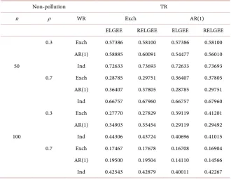
In order to study the problem (1), we compared the mean squared error of the estimating method (RELGEE) and the ordinary element empirical likelihood method (ELGEE) in the case of no pollution. The simulation results are shown in Table 1.
When processing non-polluting data, due to the robust processing of the lon-gitudinal data to some extent, resulting in the loss of part of the information, the efficiency of robust estimation is usually lower than the non-stable estimate when there is no pollution. Table 1 shows that the mean square error of RELGEE estimator is only slightly larger than that of ELGEE estimator, which shows that this method is efficient even in the case of no pollution.
[image:8.595.209.540.456.711.2]In order to explore questions (2) and (3), we have designed three ways of pol-lution:
Table 1. Comparison of Two Estimators under Non-pollution Conditions.
Non-pollution TR
n ρ WR Exch AR(1)
ELGEE RELGEE ELGEE RELGEE 0.3 Exch 0.57386 0.58100 0.57386 0.58100
AR(1) 0.58885 0.60091 0.54477 0.56010 50 Ind 0.72633 0.73693 0.72633 0.73693 0.7 Exch 0.28785 0.29751 0.36407 0.37805 AR(1) 0.36407 0.37805 0.28785 0.29751 Ind 0.66757 0.67960 0.66757 0.67960 0.3 Exch 0.27770 0.27829 0.39119 0.41201 AR(1) 0.34903 0.35454 0.29119 0.29492 100 Ind 0.44306 0.43724 0.40696 0.41015 0.7 Exch 0.17467 0.17678 0.16708 0.16904 AR(1) 0.19500 0.19504 0.14110 0.14566 Ind 0.42543 0.42879 0.40011 0.42267
DOI:10.4236/jamp.2019.76094 1416 Journal of Applied Mathematics and Physics
(C1). Pollution of the response variable Y: randomly turn S% of yij into ij
y +b, b~N
( )
2,1 .(C2). Pollution only for covariate X: randomly turn S% of xij into xij +a,
(
)
(
T)
3
~ 1,1,1 ,
a N I .
(C3). Simultaneous contamination of X and Y: randomly turn S%/3 of yij
into yij+b , b~N
( )
2,1 , randomly turn S%/3 of xij into xij+a ,(
)
(
T)
3
~ 1,1,1 ,
a N I .
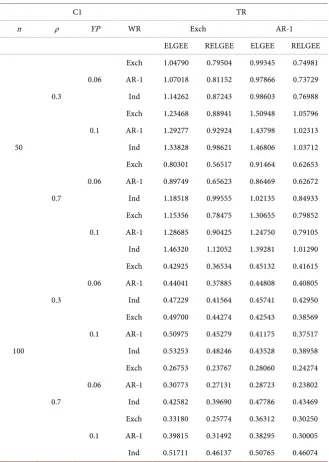
[image:9.595.210.540.250.713.2]Where S% is pollution rate. In this paper, 0.06 and 0.1 are selected. Some si-mulation results are shown in Tables 2-4.
Table 2 is the simulation results under C1. By comparison, in most cases, the
Table 2. Comparison of Two Estimators under C1.
C1 TR
n ρ YP WR Exch AR-1
ELGEE RELGEE ELGEE RELGEE Exch 1.04790 0.79504 0.99345 0.74981 0.06 AR-1 1.07018 0.81152 0.97866 0.73729 0.3 Ind 1.14262 0.87243 0.98603 0.76988 Exch 1.23468 0.88941 1.50948 1.05796 0.1 AR-1 1.29277 0.92924 1.43798 1.02313 50 Ind 1.33828 0.98621 1.46806 1.03712 Exch 0.80301 0.56517 0.91464 0.62653 0.06 AR-1 0.89749 0.65623 0.86469 0.62672 0.7 Ind 1.18518 0.99555 1.02135 0.84933 Exch 1.15356 0.78475 1.30655 0.79852 0.1 AR-1 1.28685 0.90425 1.24750 0.79105 Ind 1.46320 1.12052 1.39281 1.01290 Exch 0.42925 0.36534 0.45132 0.41615 0.06 AR-1 0.44041 0.37885 0.44808 0.40805 0.3 Ind 0.47229 0.41564 0.45741 0.42950 Exch 0.49700 0.44274 0.42543 0.38569 0.1 AR-1 0.50975 0.45279 0.41175 0.37517 100 Ind 0.53253 0.48246 0.43528 0.38958 Exch 0.26753 0.23767 0.28060 0.24274 0.06 AR-1 0.30773 0.27131 0.28723 0.23802 0.7 Ind 0.42582 0.39690 0.47786 0.43469 Exch 0.33180 0.25774 0.36312 0.30250 0.1 AR-1 0.39815 0.31492 0.38295 0.30005 Ind 0.51711 0.46137 0.50765 0.46074
DOI: 10.4236/jamp.2019.76094 1417 Journal of Applied Mathematics and Physics
Table 3. Comparison of Two Estimators under C2.
C2 TR
n ρ XP WR Exch AR-1
ELGEE RELGEE ELGEE RELGEE Exch 12.91886 0.99187 13.97928 1.02373 0.06 AR(1) 12.82331 0.99716 14.12307 1.02851 0.3 Ind 13.06875 1.03024 13.80362 1.00403 Exch 42.76916 3.00972 39.56463 2.88551 0.1 AR(1) 43.36231 3.05236 39.30508 2.88421 50 Ind 43.31341 3.05817 40.03126 2.89432 Exch 14.44630 0.88005 13.3182 0.89685 0.06 AR(1) 14.57675 0.93714 13.72404 0.87365 0.7 Ind 14.76241 1.09283 13.10561 0.93932 Exch 39.52561 2.89129 37.91395 2.73270 0.1 AR(1) 40.71029 3.08226 37.78436 2.74435 Ind 40.76240 3.18213 39.59294 2.85362
XP: Pollution probability of covariate X.
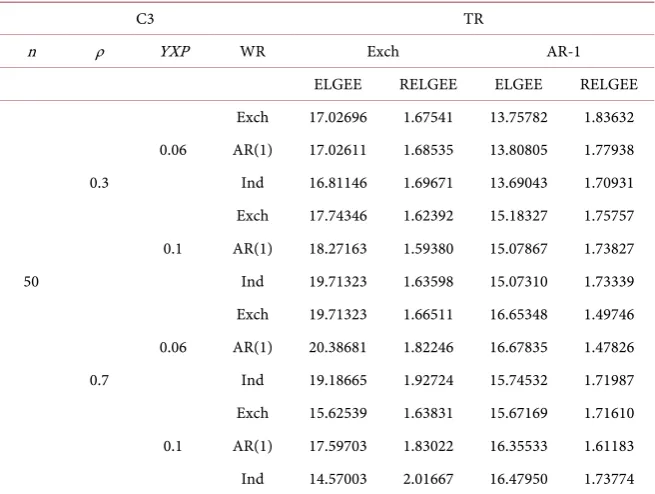
Table 4. Comparison of Two Estimators under C3.
C3 TR
n ρ YXP WR Exch AR-1
ELGEE RELGEE ELGEE RELGEE Exch 17.02696 1.67541 13.75782 1.83632 0.06 AR(1) 17.02611 1.68535 13.80805 1.77938 0.3 Ind 16.81146 1.69671 13.69043 1.70931 Exch 17.74346 1.62392 15.18327 1.75757 0.1 AR(1) 18.27163 1.59380 15.07867 1.73827 50 Ind 19.71323 1.63598 15.07310 1.73339 Exch 19.71323 1.66511 16.65348 1.49746 0.06 AR(1) 20.38681 1.82246 16.67835 1.47826 0.7 Ind 19.18665 1.92724 15.74532 1.71987 Exch 15.62539 1.63831 15.67169 1.71610 0.1 AR(1) 17.59703 1.83022 16.35533 1.61183 Ind 14.57003 2.01667 16.47950 1.73774 YXP: Pollution probability of the response variable Y when Pollution probability of covariate X is 0.06.
[image:10.595.211.539.390.637.2]DOI:10.4236/jamp.2019.76094 1418 Journal of Applied Mathematics and Physics
has a strong robustness. It can also be seen that when the working matrix is set incorrectly, the difference of estimator is relatively small; when the working cor-relation matrix is a real matrix, the estimation efficiency is the highest; when the working matrix is independent structure (Ind), the estimation efficiency is the lowest without considering the correlation between data.
Table 3 and Table 4 are part of the results under C2 and pollution mode C3. Similar to Table 2, in most cases, the mean square error of this estimator is smaller than that of ELGEE estimator. Compared with Table 2, the mean square error of ELGEE estimator is only one-tenth of the mean square error of ELGEE estimator when the pollution intensity is significantly increased. The estimation method in this paper can significantly reduce the impact of outliers on the esti-mator. Similarly, the estimation efficiency is the highest when the working cor-relation matrix is a real matrix. When there is intra-group corcor-relation in the model, the estimation efficiency is the lowest when the correlation is neglected in the estimation, which reflects the necessity of considering the longitudinal data model.
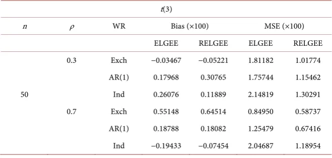
It is worth adding that because the method in this paper is a non-parametric method, the distribution of random errors does not necessarily follow the nor-mal distribution. We simulate the distribution of random errors satisfying t(3) again. The simulation results are shown in Table 5. Bias (×100) represents 100 times the deviation.
In Table 5, in all cases, the mean square error of the estimator in this paper is less than that of ELGEE estimator, which shows that the estimation method constructed in this paper can also effectively and robustly estimate the data of heavy-tailed distribution.
5. Summary
[image:11.595.209.539.570.727.2]We introduce the generalized estimating equations commonly used in longitu-dinal data, and derive robust estimation functions. Then we combine the robust estimation equations with the elemental empirical likelihood method to obtain the empirical likelihood ratio function of the estimated parameters. We show a
Table 5. The error distribution of data satisfies t(3).
t(3)
n ρ WR Bias (×100) MSE (×100)
ELGEE RELGEE ELGEE RELGEE 0.3 Exch −0.03467 −0.05221 1.81182 1.01774
DOI: 10.4236/jamp.2019.76094 1419 Journal of Applied Mathematics and Physics
relatively optimized algorithm that can improve the efficiency and computation-al time of operation. We do a systematic simulation study. The simulation re-sults show that our method maintains high estimation efficiency when the data is not polluted; in the case of data pollution, the estimator of this paper is ob-viously better than the non-robust estimator. With the increase of pollution in-tensity, the robustness of our method is more significant, and it has a significant resistance to outliers. When the working matrix is set incorrectly, the difference of estimator is relatively small; when the working correlation matrix is a real matrix, the estimation efficiency is the highest; when the working matrix is independent structure (Ind), the estimation efficiency is the lowest without con-sidering the correlation between data. At the same time, since the estimator in this paper is based on empirical likelihood method, it is suitable for the longitu-dinal data of thick-tailed distribution. There are still many problems worth fur-ther study in this paper, such as the application of estimation methods to partial linear models and variable selection based on robust estimation.
Conflicts of Interest
The authors declare no conflicts of interest regarding the publication of this paper.
References
[1] Liang, K.Y. and Zeger, S.L. (1986) Longitudinal Data Analysis Using Generalized Linear Models. Biometrika, 73, 13-22. https://doi.org/10.1093/biomet/73.1.13
[2] Diggle, P., Diggle, P.J., Heagerty, P., et al. (2002) Analysis of Longitudinal Data. Oxford University Press, Oxford.
[3] Fan, Y.L, Qin, G.Y. and Zhu, Z.Y. (2012) Variable Selection in Robust Regression Models for Longitudinal Data. Journal of Multivariate Analysis, 109, 156-167.
https://doi.org/10.1016/j.jmva.2012.03.007
[4] Huber, P.J. (1964) Robust Estimation of a Location Parameter. The Annals of Ma-thematical Statistics, 35, 73-101. https://doi.org/10.1214/aoms/1177703732
[5] Wang, X., Jiang, Y., Huang, M. and Zhang, H.P.(2013) Robust Variable Selection with Exponential Squared Loss. Journal of the American Statistical Association, 108, 632-643. https://doi.org/10.1080/01621459.2013.766613
[6] Lv, J., Yang, H. and Guo, C. (2015) An Efficient and Robust Variable Selection Me-thod for Longitudinal Generalized Linear Models. Computational Statistics Data Analysis, 82, 74-88. https://doi.org/10.1016/j.csda.2014.08.006
[7] Qin, G.Y., Zhu, Z.Y. and Fung, W.K. (2009) Robust Estimation of Covariance Pa-rameters in Partial Linear Model for Longitudinal Data. Journal of Statistical Plan-ning and Inference, 139, 558-570. https://doi.org/10.1016/j.jspi.2008.03.042
[8] Wang, Y.G., Lin, X. and Zhu, M. (2005) Robust Estimating Functions and Bias Correction for Longitudinal Data Analysis. Biometrics, 61, 684-691.
https://doi.org/10.1111/j.1541-0420.2005.00354.x
DOI:10.4236/jamp.2019.76094 1420 Journal of Applied Mathematics and Physics [10] Zheng, X., Fung, W.K. and Zhu, Z. (2013) Robust Estimation in Joint Mean? Cova-riance Regression Model for Longitudinal Data. Annals of the Institute of Statistical Mathematics, 65, 617-638. https://doi.org/10.1007/s10463-012-0383-8
[11] Owen, A.B. (1988) Empirical Likelihood Ratio Confidence Intervals for a Single Functional. Biometrika, 75, 237-249. https://doi.org/10.1093/biomet/75.2.237
[12] Azzalini, A. (2017) Statistical Inference Based on the Likelihood. Routledge, Ab-ingdon-on-Thames.
[13] Qin, J. and Lawless, J. (1994) Empirical Likelihood and General Estimating Equa-tions. The Annals of Statistics, 100, 300-325.
https://doi.org/10.1214/aos/1176325370
[14] Bondell, H.D. and Stefansk, L.A. (1994) Empirical Robust Regression via Two-Stage Generalized Empirical Likelihood. Journal of the American Statistical Association, 108, 644-655. https://doi.org/10.1080/01621459.2013.779847
[15] Bai, Y., Fung, W.K. and Zhu, Z. (2010) Weighted Empirical Likelihood for Genera-lized Linear Models with Longitudinal Data. Journal of Statistical Planning and In-ference, 140, 3446-3456. https://doi.org/10.1016/j.jspi.2010.05.007
[16] Wang, S., Qian, L. and Carroll, R.J. (2010) Generalized Empirical Likelihood Me-thods for Analyzing Longitudinal Data. Biometrika, 97, 79-93.
https://doi.org/10.1093/biomet/asp073
[17] Li, S.M., Ren, Y.Y. and Lu, G. (2018) A Robust Estimation and Empirical Likelihood Inference for Longitudinal Data Models. Journal of Applied Statistics and Manage-ment, 4, 631-638.
[18] He, X., Fung, W.K. and Zhu, Z. (2005) Robust Estimation in Generalized Partial Linear Models for Clustered Data. Journal of the American Statistical Association, 100, 1176-1184. https://doi.org/10.1198/016214505000000277
[19] Özdemir, S. and Arslan, O. (2015) An Alternative Algorithm of the Empirical Like-lihood Estimation for the Parameter of a Linear Regression Model. Communica-tions in Statistics-Simulation and Computation, 42, 1-9.