Deconvolution of the Error Associated with Random Sampling

(1)

ISSN Online: 2160-0384 ISSN Print: 2160-0368

DOI: 10.4236/apm.2019.93010 Mar. 29, 2019 205 Advances in Pure Mathematics

Deconvolution of the Error Associated with

Random Sampling

Peter L. Irwin

*

, Yiping He, Chin-Yi Chen

Molecular Characterization of Foodborne Pathogens, United States Department of Agriculture, Wyndmoor, PA, USA

Abstract

In this work empirical models describing sampling error (∆_{) are reported} based upon analytical findings elicited from 3 common probability density functions (PDF): the Gaussian, representing any real-valued, randomly changing variable x of mean µ_{and standard deviation}

σ

_{; the Poisson,} representing counting data: i.e., any integral-valued entity’s count of x (cells, clumps of cells or colony forming units, molecules, mutations, etc.) per tested volume, area, length of time, etc. with population mean of µ and σ = µ; binomial data representing the number of successful occurrences of some-thing (x+_{) out of}_n_{observations or sub-samplings. These data were}

generat-ed in such a way as to simulate what should be observgenerat-ed in practice but avoid other forms of experimental error. Based upon analyses of 104 _∆ measure-ments, we show that the average ∆₍∆) is proportional to _σ_⋅−2_n_⋅_µ−1

( 1

x

σ µ_⋅ − _{; Gaussian) or}−₂_n_⋅_µ_{(Poisson & binomial). The average}

propor-tionality constants associated with these disparate populations were also nearly identical (A=0.783 0.0470± ; ±s). However, since µ σ= for any Poisson process, ₂ 1

x n µ σ µ−

− _{⋅ =} _⋅ . In a similar vein, we have empirically

demonstrated that binomial-associated ∆ were also proportional to 1

x

σ µ_⋅ − _.

Furthermore, we established that, when all ∆ were plotted against either 2_n _µ

− _⋅ _or 1

x

σ µ_⋅ − _{, there was only one relationship with a slope =}_A_(0.767

± 0.0990) and a near-zero intercept. This latter finding also argues that all ∆, regardless of parent PDF, are proportional to 1

x

σ µ_⋅ − _{which is the}

coeffi-cient of variation for a population of sample means (C xV

[ ]

). Lastly, we

es-tablish that the proportionality constant A is equivalent to the coefficient of variation associated with ∆ ₍ C_V  _{ }∆_j _{) measurement and, therefore,}

[ ]

V j V

C   C x

∆ = _{ }∆ ⋅ . These results are noteworthy inasmuch as they provide

How to cite this paper: Irwin, P.L., He, Y. and Chen, C.-Y. (2019) Deconvolution of the Error Associated with Random Sam-pling. Advances in Pure Mathematics, 9, 205-227.

https://doi.org/10.4236/apm.2019.93010

Received: February 11, 2019 Accepted: March 26, 2019 Published: March 29, 2019

http://creativecommons.org/licenses/by/4.0/

(2)

DOI: 10.4236/apm.2019.93010 206 Advances in Pure Mathematics a straightforward empirical link between stochastic sampling error and the aforementioned CVs. Finally, we demonstrate that all attendant empirical

measures of ∆_{are reasonably small (e.g.,} 1_{~ 4%}

x

s x_⋅ − _{) when an}

environ-mental microbiome was well-sampled: n = 16 - 18 observations with µ~ 3

isolates per observation. These colony counting results were supported by the fact that the two major isolates’ relative abundance was reproducible in the four most probable composition observations from one common population.

Keywords

Stochastic Sampling Error, Modeling, Most Probable Composition, Quantitative Metagenomics, Food-Borne Bacteria

1. Introduction

There are various analytical procedures for enumerating organisms in environ-mental samples which diverge in their experienviron-mental approach yet are mathe-matically inter-related. Thus, if V represents the sample volume and Ve the volume occupied by a test entity of interest (e.g., colony forming units or CFUs), the probability that one particular Ve will not contain this entity at concentra-tion δ [1] is

(

1

)

e

e e

V V V _V

V V

δ _δ

 − ⋅ _{= − ⋅}

 

  ;

i.e., V Ve—maximum possible number of entities in V and V⋅δ~the actual number of objects present.

Assuming that many Ve aliquots have been combined to generate V, the probability that no organism will be contained in V is [1]

[

1

]

e

V V e P− _{= − ⋅}V δ therefore

[

]

ln ln 1 e

e V P V V δ −   = ⋅ − ⋅   . Since

[

]

2 3 4

ln 1 ~

2 3 4

ψ ψ ψ

ψ ψ

− − − − − −_

then, if ψ =Ve⋅δ,

2 2 3 3 4 4

2 2 3 3

ln ~

2 3 4

~ 1 .

2 3 4

e e e

e e

e e e

V V V

V

P V

V

V V V

V

δ δ δ

δ

δ δ δ

δ −  ⋅ ⋅ ⋅    _− ⋅ − − − − _      ⋅ ⋅ ⋅  − ⋅ _ + + + + _    

(3)

DOI: 10.4236/apm.2019.93010 207 Advances in Pure Mathematics

ln_{  − ⋅}P− ~ V

δ

 

[

]

[ ]

exp exp

P− ₌ _{− ⋅}V δ ₌ ₋µ

therefore

[

]

[ ]

1 1 exp 1 exp

P+ _{= −}P−_{= −} _{− ⋅}V δ _{= −} ₋µ _{. (1)} In certain circumstances it is only possible to determine an organism’s δ by diluting the sample to such an extent that only a fraction of the n “technical” replicates tested are positive (x+_{) for the presence of the entity, or microbe, in}

question [3][4]. This technique is referred to as the “dilution method” [1] since it involves diluting a test sample’s content to extinction (δ →0_{). This}

enumera-tion protocol is also known as the most probable number (MPN) method and entails sampling from a liquid source, making serial dilutions from this, distri-buting an aliquot of each of these dilutions into separate receptacles, incubating these under suitable growth conditions, and observing if any growth has oc-curred based upon some organism-specific detection method [5][6]. The MPN

enumeration procedure is particularly useful when sampling from environmen-tal sources, such as foods, since damaged cells frequently recover in liquid media [7].

For example, were one to obtain a food sample containing ~14 CFU of a par-ticular organism per 50 g, the cells would typically be washed from the food ma-trix, concentrated to a few mL (e.g., via centrifugation), and brought up to some appropriate volume (say 40 mL = Vsample) with media [5]. From this, eight 4 mL (V) samples could be randomly selected and distributed into 8 separate recep-tacles (n = 8 with a dilution factor of 1; i.e., undiluted). Of the remaining 8 mL, 4 could be further diluted with 36 mL (40 mL total) liquid media, mixed and dis-tributed into another set of 8 containers. This set of dilutions has a dilution fac-tor of 0.1 relative to the original. With the remaining 8 mL from the 0.1 dilution, 4 mL could be diluted again with 36 mL media, mixed and distributed into yet another eight 4 mL replicates (dilution factor = 0.01). After incubation the most likely number (Equation (2), below) of positive occurrences (e.g., presence of a specific gene [5]) observed would be x+_{= 6, 1, and 0 (out of}_n_{= 8 observations}

per dilution) for dilution factors of 1, 0.1, and 0.01, respectively, and the calcu-lated MPN (±s) per 50 g sample would = 13.8 ± 5.56. Note the relatively large error term. For a 4-fold proportional (200 g, 160 mL Vsample) experiment with n = 32, the calculated MPN is 13.8 ± 2.78 per 50 g sample.

For MPN-based organism detection and subsequent enumeration, the number of positive occurrences of growth in any jth_{experiment out of}_n_{observations =}

1 n

j i ij

x+

θ

=

∑

₍_θ_{= either 1 [presence] or 0 [absence]) can be estimated as}

[

]

(

)

~ 1 exp

x+ n P_⋅ + ₌n ₋ _{− ⋅}V

δ

(2) whereupon x+_{is integral (=ROUND(}_{n P}_⋅ +_{, 0) in Excel). The probability of}

observing x+ _{successes out of}_n_{Bernoulli trials}_[8]_{each of volume}_V_{from a}

(4)

(

!

) ( ) ( )

! !

n x x

b n

P P P

x n x

+ + − − + + + = −

which is also known as the binomial PDF. Since n P_⋅ +_{= the population average}

(real) [9] number of positive responses out of n tests (µ+_{), the above can be also}

written as

(

!

)

1

! !

n x x

b n

P

n n

x n x

µ+ −+ µ+ +

+ +

   

= _ − _ _ _

− _ _ _ _ . (3) The multiple dilution MPN calculation itself is determined by finding the val-ue of

δ

at the maximum in the product of the P sb from all th dilutions (

∏

Pb, ) and is easily achieved by adding the scaled sum of all dilutions’

b b

P P

δ

∂ ÷ _{values to an initial guess for}

δ

(i.e.,

{

}

(

)

(

)

(

)

{

}

1 , ,

exp 0.1 1 0.1

m m m b b _m

m m m

P P

x n x V V

δ

δ δ λ

δ λ δ

+ + + = + × ∂ ÷   = + × − + ÷ _ ⋅ ⋅ _− ⋅ ⋅

∑

      

 for any particular

ℓ th_{one-to-ten dilution and}_m_iterations;_λ_{is a monotonically changing, with}_m_, scaling function) then solving for the MPN recursively [1] [4] [5] [10] which minimizes the summation.

At the limit n → ∞, Equation (3)simplifies to what is known as the Poisson

PDF

[ ]

exp ! x P P x

µ −µ

= _{. (4)} Under these circumstances, x is the observed and µ_{is the population average} number of counts in/on the tested volume, surface, chosen time period, etc. This

PDF is applicable to all analytical systems involving, essentially, the counting of objects. However this PDF is applied, the most conspicuous aspect [11][12] of any Poisson process is that the variance (_σ2_{or second moment)}

(

)

2

0 P

x x P

σ ∞ µ µ

=

∑

− =

equals the population mean (µ_{or first moment)}

0 P x x P µ ∞ = =

∑

⋅ .

The last probability density function utilized in this stochastic sampling exer-cise is also related to Pb, Equation (3). This is the Gaussian PDF which we use to quantitatively examine the effects of n and

σ

(fixed µ_{) on the variability of} sample means (x) which have been created by randomly sampling from a pop-ulation of real-valued variables (x; e.g., doubling time [13]) which are normally distributed as

2

Area _exp 1

2 2π G x P

µ

σ

 _ ₋ _  = − _ _   

 ; (5) in this relationship the Area term (~ 1

K k k

x = f

(5)

DOI: 10.4236/apm.2019.93010 209 Advances in Pure Mathematics area under the fitting function f (frequently taken to be 1 since ∆x is often = 1 and

∑

f is always ~1). There are several derivations of PG but none are as persuasive as the fact that this PDF is simple and has been experimentally shown to be the most likely probability distribution associated with most experimental observations [9][12].

The original purpose of our sampling-related investigations [7] was to esti-mate a nominal value for n needed to achieve accurate most probable foodborne bacterial isolate enumeration, combined with 16S rDNA-based identification, for quantitative metagenomic purposes. The relationships were developed by examining the results of 6 × 6 colony counting (Poisson PDF) of highly diluted bacteria [14][15] as a function of n and µ_{as well as by generating counts (}_x₎ derived from PP to simulate what occurred in the lab [15] [16] but which avoided other forms of experimentally based error [5]. We were able to establish

that 3

min 1

n =nµ→ ÷ µ where nµ→1 is the number of observations necessary to accurately enumerate a population average of 1 count per volume tested. Based mainly on colony counting experience we estimate nµ→1 is somewhere in the range n ~ 20 - 30 observations.

Herein we model stochastic sampling errors associated with all the aforemen-tioned PDFs and empirically demonstrate that the resultant mathematical mod-els are, in part, a consequence of the “central limit theorem” [17] (CLT). In gen-eral, the CLT states that a distribution of sample means (x), regardless of parent

PDF, approaches a normal distribution analytically equivalent to PG, Equation (5), with x x= , µ µ= x, and with the σ2 term = σ2x (= σ ÷2 n) as the

number of separate n-samplings increases. We also have elaborated on empirical findings developed previously [5][15][16] for predicting errors associated with the random sampling of microorganisms as well as comparing the internal vari-ations associated with the three different sampling error data types derived from the Gaussian, binomial (MPN), and Poisson relationships. Thus, new results have been created using the aforementioned probability distributions, Equations (2), (4), and (5), and have been highly replicated since each “experiment”, com-prising n (= 3, 6, 9, 12, or 24) observations, were repeated 100 times.

2. Materials and Methods

2.1. Poisson-Based Data: Equation (4),

Figure 1

All counting data were created by multiplying Equation (4) by 360 in order to produce a large number of integral-valued repeats (=ROUND (360⋅PP, 0)) for any particular count x: e.g., for µ =1 particle per test volume, area, length of time, etc., there would be, most probably, 132 repeats of x = 0, 132 repeats of x = 1, 66 repeats of x = 2, 22 repeats of x = 3, 6 repeats of x = 4 and 1 repeat of x = 5 entities per test. From this pool of 360 counts for each μ, an n number of x val-ues were randomly selected based upon random number tables created with

Mathematica.

{

} { }

(6)

[image:6.595.64.537.73.327.2]

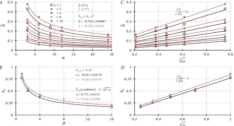
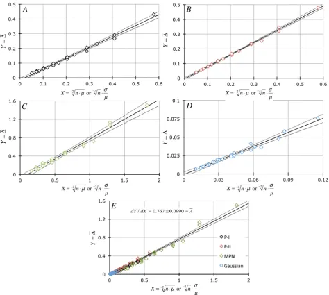
Figure 1. (A) relationship of average ∆j (∆) for Poisson-based data using Equation (7) (P-I: black symbols and curves) or

Equ-ation (8) (P-II: red symbols and curves) as a function of n (= 3, 6, 9, 12, 24) and various values for μ (= 1, 2, 4, 8, 16). Gauss-Newton least squares minimization-based curve-fitting [18] of data was performed [19] to fit to the equation a

n n ∆ = ∆ ⋅ (averages for a are provided ± s; averaged across 5× μ). (B) Non-linear relationship of individual ∆n values from (A) for P-I- and

II-based data as a function of μ whereupon curve-fitting of data was also performed using the algebraic form a n A µ

∆ = ⋅ (values

for A and a are provided ± ASE). (C) and (D) Present linearized forms (_X ₌−2_n_{in (C) and} _X ₌−2_µ_{in (D)) of data reported}

in Figure 1(A) and Figure 1(B) based upon all values of a = −1/2. Slopes of the lines in Figure 1(C) and Figure 1(D) are

equiva-lent to ∆n and A, respectively.

which generates n random numbers between 1 and 360. Thus, 100 such random number sets were utilized for the twenty-five n (= 3, 6, 9, 12, 24) × μ (= 1, 2, 4, 8, 16) combinations. Briefly, each procedure involved arranging the aforemen-tioned 360 x values (one set for each μ) in one column of a spreadsheet followed by filling in n adjacent columns with formulae which refer to the calculated x

values but where each row’s reference number was taken from the Mathemati-ca-generated random number, Equation (6), next in sequence. MPN- and Gaus-sian-based data arrays were treated in an identical fashion. The formula (P-I: normalized deviations of sj from σ = µ ) for calculating our empirical measure of Poisson stochastic sampling error (Δ) was

j j

s

µ

−

∆ = ₍₇₎ whereupon the sj term is the experimental standard deviation (

(

)

1

(

)

2

1

1 ni ij j

n − x x

=

−

∑

− or “=STDEV.S (xij-array)” in Excel) for each j th

( j=1, 2, , J; J = 100) experiment and i th₍_i₌_{1,2, ,}_ _n₎_x_{. The average across}

(7)

DOI: 10.4236/apm.2019.93010 211 Advances in Pure Mathematics 1

1

J j j J−

=

⋅

∑

∆ or “=AVERAGE (∆j-array)”). A second form for the

Pois-son-based measure of Δ was also calculated (P-II: normalized deviations of xj from known μ) from these same data

j j

x

µ µ −

∆ = . (8)

Here the xj is the observed arithmetic mean for each j th counting experi-ment.

2.2. MPN Experiments: Equation (1), Figure 2

All MPN data were created by multiplying Equation (1) by 360 to produce the number (“=ROUND (360_⋅P+_{, 0)”) of positive responses (}_θ_{= 1) for any}

partic-ular level of V⋅δ (=μ); e.g., for µ=0.1 entity per volume tested there would be 34 repeats of θ = 1 and 326 repeats of θ = 0. From such a column of 360 θ

[image:7.595.58.534.338.615.2]

values (one column for each μ), n were randomly selected based upon Mathema-tica tables, Equation (6), and treated similar to the Poisson data above. Thus, for each combination of n (= 3, 6, 9, 12, or 24) × μ (= 0.1, 0.2, 0.4, 0.8, 1.6), 100

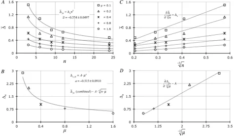
Figure 2. (A) Relationship of average ∆j (∆) for MPN-based data using Equation (9) as a function of n (= 3, 6, 9, 12, or 24) and

variable μ (= 0.1, 0.2, 0.4, 0.8, 1.6). Gauss-Newton least squares minimization-based curve-fitting [18] of data was performed [19] to fit the algebraic form a

n n

∆ = ∆ ⋅ (averages for a are provided ± s; averaged across 5 × μ) to these results. (B) Relationship of

individual ∆n values from (A) for MPN-based data as a function of μ where curve-fitting of data was performed also to the alge-braic form a

n A µ

∆ = ⋅ (values for A and a are provided ± ASE). (C) and (D) Represent linearized forms (_X ₌−2_n_{in (C) and}

2

X₌− µ_{in (D) of data reported in}_{Figure 2(A)}_and_{Figure 2(B)}_{based upon the assumption that}_a_{= −1/2. Slopes of the lines in}

(8)

DOI: 10.4236/apm.2019.93010 212 Advances in Pure Mathematics random n-selections were performed. The formula for calculating our empirical measure of MPN sampling error was

1 n

ij

j i

j

n P _x

n P

θ _µ

µ

+

+ +

=

+ +

⋅ − ₋

∆ = =

⋅

∑

; (9)

where θ = either a “1” (a positive occurrence) or a “0” (a negative occurrence). As before, the average ∆j across J = 100 experiments (each of n observations) =∆. The MPN value for x+j =ln_n n x÷ −

(

+j

)

_ and provides the average MPN

or CFU per sample; a rearrangement of Equation (2).

2.3. Gaussian-Based Data: Equation (5), Figure 3

[image:8.595.60.533.349.633.2]

All Gaussian PDF data were produced by multiplying Equation (5) (∆ =x 1) by 360 producing an integral number of observations (“=ROUND (360⋅PG, 0)”) for each value of x as a function of μ (fixed at 20) and σ (= 1, 1.5, 2, 3, 4). For in-stance, for σ = 1 there would be 2 repeats of x = 17, 19 repeats of x = 18, 87 re-peats of x = 19, 144 repeats of x = 20, 87 repeats of x = 21, 19 repeats of x = 22, and 2 repeats of x = 23. From this column of 360 values of x, n (= 3, 6, 9, 12, or

Figure 3. (A) Relationship of average ∆j (∆) for Gaussian-based data using Equation (10) as a function of n with variable σ

(=1, 1.5, 2, 3, 4; μ = 20). Gauss-Newton least squares minimization-based curve-fitting [18] of data was performed [19] to fit the equation a

n n

∆ = ∆ ⋅ (averages for a are provide ± s; averaged across 5× σ) to these results. (B) and (D) Relationship of individual

n

(9)

DOI: 10.4236/apm.2019.93010 213 Advances in Pure Mathematics 24) were randomly selected based upon Equation (6) and treated identically to the Poisson and MPN data sets. Thus, for each combination of n × σ 100×

n-based selections were performed. The formula for calculating our empirical measure of Gaussian sampling error, similar to Equation (7), was

j j s σ µ −

∆ = _{. (10)}

As usual, the average ∆j across J = 100 such sets of experiments each of n observations = ∆_.

2.4. Other Calculations

All curve-fitting was based upon a modified Gauss-Newton algorithm by least squares [18] minimization performed on a Microsoft Excel spreadsheet: [19] some of these results were fit to the algebraic form _{f X}

[ ]

₌constant_⋅_Xa_.

How-ever, certain MPN data (x+_and _x+_{) were also fit to a Gaussian (Equation (5):}

G

P x_{ }+

  or P xG  + ) with ∆x used as one of the parameters to be iteratively resolved (i.e., deconvolved). Where appropriate, confidence limits (CL) have been calculated using an approach applicable to any hypothetical fitting function

;

k k p

f _{= }f X

π

__: _k=_{1, 2, ,} _K rows of the observed X-Y data sets with up to P

(typically ≤ 3) fitting parameters

π

p (p=1, 2, , P). In this procedure we use the propagation of error method [9][20] for estimating the standard error asso-ciated with each fk (sfk ; illustrated below for P = 2 fitting parameters) data

point

1 1 2 2 1 2 1 2

2 2

2 ₂2 2

k

f k k k k

t s t s f s f f f

CL= ⋅ = π ∂π  + π ∂π  + ⋅sπ π ⋅ ∂π ⋅ ∂π

where, for any particular fitting parameter

ω

, 2 T 1

Y

sω s _ωω

−

 

= _{⋅ }Z Z_ = “asymp-totic standard error” [19] (ASE; 2

Y

s = residual sum of squares ÷ [K − P]), and the ∂π_pfk terms symbolize ∂ ∂fk

π

p. The above equation simplifies to

(

1

)

2 T T

0.01 fk 0.01 Y k k

t

CL= ⋅s =t s Z Z Z_ _− Z .

In all the above relationships Z is the partial first derivative matrix of fk with respect to the parameters π1 and π2 (i.e., a 2-parameter fit) such that

1 2 1 2 1 2 1 1 2 2 K K f f f f f f π π π π π π ∂ ∂     ∂ ∂   =     ∂ ∂    Z   , T

Z is the transpose of Z, Zk = ∂ π₁fk ∂π₂fk (K row vectors), and 1

2 T

Y

s _{⋅ }_{Z Z}_− _{is the variance-covariance matrix}_[21]_._CL_{were not used for all} results since they might have muddled analytical aspects of the compositions.

2.5. Microbiome Sampling Data

(10)

DOI: 10.4236/apm.2019.93010 214 Advances in Pure Mathematics (~15 min at room temperature), frozen vegetables were washed with a volume of phosphate buffered saline (PBS; 10 mM Na2HPO4 + 2 mM NaH2PO4 + 137 mM NaCl; pH 7.4 ± 0.2; Boston BioProducts, 159 Chestnut Street, Ashland, MA 01721) equivalent to double the mass of the sample. In order to assist in the de-tachment of plant tissue-bound cells, 0.075% [w/v] Tween-20 (Sigma-Aldrich, 3050 Spruce St., St. Louis, MO 63103) was added to the PBS and filter sterilized. All washing was performed in sanitized plastic zip-lock bags wherein the for-merly frozen vegetables and buffer wash were gently agitated at 80 rpm for ap-proximately 20 min and immediately passed through a 40 μm nylon filter (BD Falcon; Becton Dickinson Biosciences, Bedford, MA) to remove large particles.

Directly sampled washes (5 mL Control = Observation I [cultured at 30˚C] and III [cultured at 37˚C]) as well as hollow fiber microfilter-concentrated (each 5 mL sample was diluted to ~100 mL PBS + Tween, concentrated, then washed with another 100 mL buffer, and eluted with ~5 mLs PBS + Tween = Observa-tion II [cultured at 30˚C] and IV [cultured at 37˚C]) samples were collected and enumerated using the 6 × 6 drop plate method [14] but using 1:2 serial dilutions for colony selection on Brain Heart Infusion agar (BHI + 2% [w/v] agar). Briefly, this drop plate method involved loading 400 μL of each wash (either control or concentrated samples brought back to the control sample’s original volume = 5 mL) filtrate into the first well (row A) of a 96-well microtiter plate. Two-fold serial dilutions were made by transferring 200 μL (multichannel pipette, Rainin, Emeryville, CA) from the first row (row A; dilution 0) into 200 μL of diluent (PBS) in the 2nd row (row B; dilution 1), mixing 10 times while continuously stirring, and repeating the process until five 1:2 dilutions were produced; pipette tips were changed between dilutions. Based on a previous analysis of 6 × 6 drop plate sampling error [15], we sampled n = 16 - 18 seven μL volumes from each of the 6 dilutions (dilutions 0 - 5; overall dilution factors of 0.50_{= 1 to 0.5}5₌ 0.03125) and drop-plated these onto BHI agar media using a multichannel pi-pette. After plating, the droplets were allowed to dry, inverted and then incu-bated at two temperatures (either 30˚C or 37˚C; 3 plates for each temperature and treatment combination). Colonies were counted after 16 - 24 hours. Colony collection for our 16S rDNA bacterial identification protocol [7] involved se-lecting all colonies from dilution 2 (0.52_{= 0.25 dilution;} _x_{= 2.79 ± 1.52} colo-nies per drop; ± s; the fact that x = 1.67 ~ s might argue for an appropriately sampled population).

(11)

DNA amplification step (end-point PCR). Once the 16S rRNA “gene” amplifica-tion, sequencing reactions (EubA and EubB primers) and Sanger sequencing were performed, DNA sequences were edited, and contigs assembled using Se-quencher software as explained in detail previously [7].

3. Results and Discussion

Figure 1 shows results related to averages of 100 × ∆j values (∆) derived from Equations (7) (P-I, black data) or (8) (P-II, red data) as a function of n (Figure 1(A)) and μ (Figure 1(B)). The least squares curve-fitting results show that the Figure 1(A) data follow the general form a

n n

∆ = ∆ ⋅ whereupon a (averaged across 5 n-based fits) = −0.556 ± 0.00986 (black data sets; ±s) or

0.529 0.0387

a= − ± (red data). These findings suggest that ∆ changes as the inverse square root of n for all values of μ. Figure 1(C) displays these same re-sults on a linearized scale (X-axis = −2_n _{) whereupon the slopes}

(

2

)

_~

n n −

 

∂∆ ∂_ _ ∆ . Figure 1(B) illustrates that the ∆n values derived from Figure 1(A) non-linear regression change as the inverse square root of μ: i.e.,

a

n A µ

∆ = ⋅ _where_a_{= −0.547 ± 0.0179 (black data) or −0.503 ± 0.0374 (red} da-ta); a ± ASE. Figure 1(D) shows Figure 1(B) results plotted on an appropriately linearized scale (X-axis = −2µ ) as indicated by the above analysis whereupon the slope

(

2

)

_~

n − µ A

∂∆ ∂   . Combining results from Figure 1(A) and Figure 1(B) we see that _∆_~ _A_⋅−2_n_⋅_µ _{. The average value for}A_{was 0.804 ± 0.0460 (}P_-I & P-II curve-fitting results ±s).

Figure 2 displays MPN-based enumeration data, Equation (9), manipulated in a similar fashion as that of the above Poisson-based results with a nearly identic-al result. The least squares curve-fitting shows that the data in Figure 2(A) once again follow the general form a

n n

∆ = ∆ ⋅ _with a = −0.554 ± 0.0499 (±s) which is the average a from 5× μ-based data sets. Figure 2(C) shows these same findings graphed on a linearized scale (_X ₌−2_n_{) whereupon the slopes =}

n ∆ _. Figure 2(B) also shows that the ∆n values, derived from Figure 2(A) non-linear regression, change as the inverse square root of μ: a

n A µ

∆ = ⋅ where

a = −0.515 ± 0.0910 (±ASE). As previously observed, when these results are pre-sented on a linearized scale (_X ₌−2µ_;_{Figure 2(D)}_{) the slope is equivalent to} the parameter A. Combining fitting results from Figure 2(A) and Figure 2(B) we again note that _∆_~_A_⋅−2_n_⋅µ (A = 0.807 ± 0.139; ± ASE).

Completely homologous relationships to the Poisson and MPN findings were also noted with Gaussian-based data (Figure 3) whereupon the least squares curve-fitting in Figure 3(A) shows that these data obey, again, the general form

a n n

∆ = ∆ ⋅ whereupon a = −0.561 ± 0.0276 (±s; averaged across all σ since μ

was fixed). Figure 3(C) has these same findings plotted on a linear scale (_X ₌−2µ) where the slopes =

n

(12)

[ ]

1 1

2

x V

A σ − n µ− A σ µ− A C x

∆ = ⋅ ⋅ ⋅ = ⋅ ⋅ = ⋅ whereupon C xV

[ ]

is the

coeffi-cient of variation for a population of means associated with x.

3.1. Equivalence of Sampling Errors Associated with Any PDF

The counting results alluded to above (P-I, P-II, & MPN) are similar to those observed previously: [5][15][16]i.e., stochastic sampling errors associated with microbiological colony counting and MPN data are proportional to the inverse square root of n × μ. Also, the Poisson population-based results compare favora-bly with those obtained from actual colony counting experiments [14]. Thus, for all Poisson-based data (Figure 1)

[ ]

1 1

1 x

V

C n

n n x

µ σ σ

µ µ

µ ⋅ = µ

∆∝ = ⋅ = =

⋅ (11)

[image:12.595.60.532.368.650.2]

because σ = µ_{. We have simplified the expression by utilizing the term}σ_x [22] (=σ ÷ n) which can be derived using the propagation of errors method [20]. Such nomenclature exemplifies the utilization of PG, as an approximation for PP, associated with a population of sample means (x) of mean µx and standard deviation σx. However, for MPN results, does σ ~ µ as an ap-proximation? This question is addressed in detail (Figures 4-6).

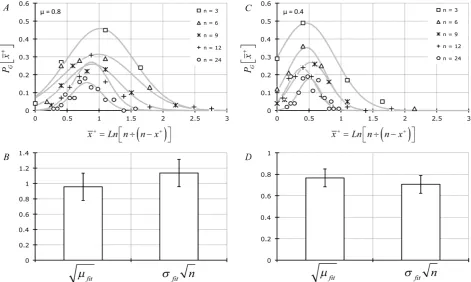
Figure 4. (A) & (C) Frequency of observing each set of MPN-based calculated number of entities per sample tested

(x+₌ln_n n x_÷

(

₋ +

)

_

 ; μ = 0.8 for (A) & (B); μ = 0.4 for (C) & (D) fit to Equation (5) (i.e., P xG  + as a function of x +

(13)

[image:13.595.246.493.75.558.2]

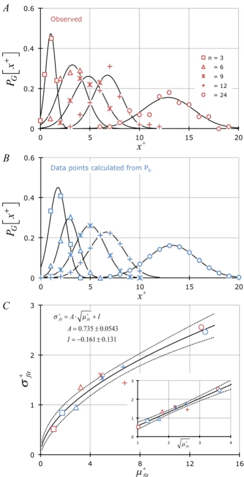
Figure 5. (A) & (B) Frequency of observing each set of MPN-based

number of positive counts x+_tested:_μ_{= 0.8 and}_n_{= 3, 6, 9, 12,} 24; (A) data points [red] = frequency of observed x+_{, (B) data} points [blue] = calculated frequency of x+_using_Mathematica

( ) (

)

(

)

{

}

e 1 e !

Table , ,0, 1

! !

n x x

b

n

P x N x n

n x x

µ −+ µ +

− −

+ +

  ₋  

   

  = +

  _ _ ₋ _ _

 

   

 

from Pb,

Equation (3), fit to a Gaussian probability distribution: e.g.,

G

P x_{ }+

 , Equation (5). (C) Demonstrates that σfit µfit + _∝ +

. Linear fit showing slope (A) and intercept (I) ± ASE. The non-linear fits were σfit A

( )

µfit 0.550 0.0463

±

(14)

[image:14.595.59.534.72.497.2]

Figure 6. Demonstration that _{d d}

(

)

_{~ ~ d d}

(

2

)

x A n

σ µ − µ

∆ ∆ ⋅ _{. All data are plotted ±}_P_{= 0.001}_CL_{. (A) is related to}_P-I_{data (}_A₌ 0.741 ± 0.0203; ± ASE). (B) is related to P-II data (A = 0.827 ± 0.0133). (C) is related to MPN data (A = 0.861 ± 0.0273). (D) is related to Gaussian data (A = 0.637 ± 0.0280). All data are merged in (E): slope of this relationship which involves all three PDFs is 0.767 ± 0.0990.

In Figure 4(A) and Figure 4(C), we have examined some of our MPN data (μ = 0.8 per sample in Figure 4(A) and μ = 0.4 per sample in Figure 4(C) at the various levels of n-sampling) by converting the total number of positive occur-rences (x+j) in n observations to the most probable number of entities in the

hypothetical sampled aliquot (x_j+ ₌ln_n n x

(

₋ +_j

)

_

 ) and curve-fit the frequency of occurrence of each xj+ to Gaussian PDFs (Equation (5); P xG  + ). From these curve fits we extracted the parameters

σ

fit and

µ

fit. In Figure 4(B) and Figure 4(D) we show that the average

σ

fit n~

µ

fit (i.e.,

fit fit n x

(15)

DOI: 10.4236/apm.2019.93010 219 Advances in Pure Mathematics approximation. We have confirmed the MPN results in Figure 2 and Figure 4 by showing that the frequency distribution of x+_{which we have observed in}

these experiments closely follows Equation (3) (compare Figure 5(A) with Fig-ure 5(B)) whereupon we establish that σfit+ , the standard deviation associated

with the distribution of x+_{via the Gaussian approximation, was proportional}

to µ+fit (Figure 5(C)) for both observed (red data) and calculated (blue data)

x+_{with a proportionality constant numerically similar to}_A_{(=0.735 ± 0.0543;}

±ASE) alluded to above.

The equality in Equation (11) is also visually confirmed by the results shown in Figure 6 where one can see that all values of ∆ closely follow the linear ex-pression ∆ = ⋅A X (for X =σx÷µ or −2n⋅µ; A = 0.781 ± 0.0107; ±ASE) showing that

[

]

2_n µ σ_x µ

−

∂∆ ₌ ∂∆

∂ ÷

 

∂_ ⋅ _ .

Since the combined data in Figure 6 are linear with a near-zero intercept (−0.0168 ± 0.00443), then

2

x

n µ σ µ

−

∆ ₌ ∆

÷ ⋅

therefore cross-multiplying gives

x n

σ µ µ

∆ ⋅ ÷ = ∆ ⋅ ⋅ and dividing both sides by ∆ produces the equality

2

x n

σ

_{÷ =}

µ

− _⋅

µ

_.

All sampling error-related findings are summarized in Figure 7.

3.2. Demonstration That

 

_{ }

j V j

A

= ∂

s

∆

∂∆ =

C

∆

Lastly, all these assertions are substantiated by the observation (Figure 8) that the standard deviations associated with all our sampling error measurements (s∆_j) change linearly as a function of the 4 (P-I, P-II, MPN, Gaussian) sets of ∆

data with an average slope (i.e., average of the 4 ∂s∆j ∂∆ values = 0.716 ±

0.0739) equivalent to the various values for A in Figures 1-3, Figure 5 and Fig-ure 6. In fact, the slope in Figure 8 defines the coefficient of variation in ∆ (CV  ∆j ) and, if equal to A, then

j

s X

∆

∂ _∂∆

=

∂∆ ∂ (12) where X = either −2_n_⋅µ_or

x

σ ÷µ_{. Since} j

s∆ in Figure 8 and ∆ in Figure

6 are linear functions with a near zero intercept then, assuming Equation (12) is true,

j

s X

∆ ∆

(16)

[image:16.595.211.536.74.347.2]

Figure 7. Summary of curve-fitting results associated with each PDF and method for

calculating empirical stochastic sampling error (∆). Each constant of proportionality A is presented ± ASE. For binomial data (MPN) µ= ⋅V δ (the population average number of entities in V) and n P_⋅ +₌µ+_{(the population average number of positive responses} out of n observations).

j

s _{A X}

A X X

∆ ⋅

= ⋅

2 j

s A X

∆

=

(

)

2

j

s∆ =A X A A X⋅ = ⋅ = ⋅ ∆A

and therefore

j

V j A

s C ∆

 ∆ 

= _=

∆

The above equality establishes that the coefficient of variation associated with ∆ (CV  ∆j ) is equivalent to the proportionality constant A seen in Figures 1-3 and Figure 6. Thus sampling errors can be estimated from the relationship

[ ]

V j V

C   C x

∆ = _{ }∆ × _whereupon CV  ∆j ~ 0.75 for all PDFs we have tested.

3.3. Minimized Errors Associated with a Well-Sampled Food

Microbiome via Most Probable Composition

[7]

(17)

[image:17.595.62.534.73.520.2]

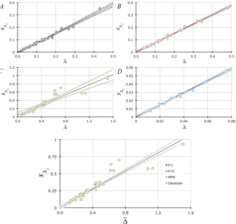
Figure 8. (A)-(D): Dependency of the standard deviation (plotted ± P = 0.05 confidence limits) derived from each experimental

j

∆ array (Y s= ∆j; j=1,2, ,25 ) on their averages (X= ∆): Figure 8(A) = P-I data (Spearman’s coefficient of rank

correla-tion: [22] ρS =0.996;

3 10

P −

 ); Figure 8(B) = P-II data (ρS =0.988;

3 10

P −

 ); Figure 8(C) = MPN data (ρS=0.979;

3 10

P −

 ); Figure 8(D) = Gaussian data (ρS=0.994;

3 10

P −

 ). The average slopes associated with these 4 relationship = 0.716 ± 0.0739 (± s). All points (25×∆ per set) from (A) through (D) are combined in the bottom-most figure (ds∆_j d∆ =0.661±0.0186 ; ± ASE). The value ds∆_j d∆ is equivalent to an experimental coefficient of variation for

V j

C  

∆ = _{ }∆ .

on commercially available, frozen vegetables were sufficiently sampled using an

n = 16 - 18 inasmuch as the C xV

[ ]

-values associated with the normalized

colo-ny counts (CFU g−1_{averaged across all}__{dilutions =} _x

 ÷ 0.007 mL per drop ÷

0.5_{dilution factor × 57.2 mL total original sample volume ÷ 28.6 g total frozen}

(18)

[image:18.595.256.503.65.533.2]

Figure 9. Estimation of the stochastic sampling errors (x÷x−1~

(19)

DOI: 10.4236/apm.2019.93010 223 Advances in Pure Mathematics similar vein, it is pertinent that the observed (s) and calculated ( x_ ) standard deviations associated with the counts per drop were equivalent since the average deviation ( s− x_ ) from ideality varied only 15.7% ± 3.54% (±sx). Lastly it is also significant that the dilution factors calculated from the ratios of average plate counts (x÷x−1) were very close to ½ (average 0.523 ± 0.0172) which also argues for a minimized ∆_.

Across the 4 observational sets (I, II, III, and IV) depicted in Figure 9, the to-tal number of collected colonies (from _=2_{) was 55 (}_n_{= 16), 49 (}_n_{= 16), 42 (}_n₌

17), and 41 (n = 18), respectively. Bacteria identifications for each of these colo-nies were based upon rDNA sequence matching 1200 - 1400 basepair contigs searching against NCBI’s GenBank database. The rRNA “gene” sequencing re-sults for the 2 major isolates (making up 88.3% ± 3.28% of the total sampled co-lonies) show that the 4 sets of observed bacterial compositions were nearly iden-tical (43.6% ± 8.05% Luconostoc and 44.6% ± 13.3% Lactococcus; ±s) [23]. The remainder of the colonies was mainly Acinetobacter (3.74% ± 3.34%) and

Strep-tococcus (4.17% ± 2.75%) with small amounts of diverse isolates (e.g.,

Staphylo-coccus, Arthrobacter, Sphingobacterium, Enterococcus, Kocuria, Raoultella, and

Bacillus: averaging 1.49% ± 1.09% each). Such variability is expected for the rela-tively rare isolates (≤4%) due to errors associated with random sampling. The

two major species sampled were relatively repeatable because of their

abun-dance, adequate sampling, and very little treatment effect. The minor constitu-ents would have to have been sampled 2.77 ± 0.647-fold more (n > 44) for an equivalent accuracy to the Luconostoc and Lactococcus fractions since the re-quisite number of samplings for the low count fractions, above, is proportional to the inverse cube root [5][16] of the number of counts per sampled volume (~

3 3

major minor

x ÷ x _).

4. Summary

We have performed analyses associated with empirical stochastic sampling er-rors linked to data generated from 3 common probability density functions. We have used these to describe the limiting behavior of ∆_{by generating models} which suggest a generalized, and facile, mathematical solution. Based upon all our experiments, the common algebraic solution, regardless of parent distribu-tion, is that experimental sampling errors are proportional to σx÷µ. This ge-neralized relationship is intuitively reasonable inasmuch as this is the CV for

anypopulation of sample means (C xV

[ ]

) and describes how closely x values

approach μ as n increases. The proportionality constant for all these findings was found to be mathematically related to CV[ ]∆j or ∂s∆j ∂∆, which is the

(20)

Conflicts of Interest

The authors declare no conflicts of interest regarding the publication of this pa-per.

References

[1] Halvorson, H.O. and Ziegler, N.R. (1933) Application of Statistics to Problems in Bacteriology. I. A Means of Determining Bacterial Population by the Dilution Me-thod. Journal of Bacteriology, 25, 101-121.

[2] Kubitschek, H.E. (1990) Cell Volume Increase in Escherichia coli after Shifts to Richer Media. Journal of Bacteriology, 172, 94-101.

https://doi.org/10.1128/jb.172.1.94-101.1990

[3] Barkworth, H. and Irwin, J.O. (1938) Distribution of Coliform Organisms in Milk and the Accuracy of the Presumptive Coliform Test. Journal of Hygiene, 38, 446-457.https://doi.org/10.1017/S0022172400011311

[4] Best, D.J. (1990) Optimal Determination of Most Probable Numbers. International Journal of Food Microbiology, 11, 159-166.

https://doi.org/10.1016/0168-1605(90)90051-6

[5] Irwin, P., Reed, S., Nguyen, L., Brewster, J. and He, Y. (2013) Non-Stochastic Sam-pling Error in Quantal Analyses for Campylobacter Species on Poultry Products. Analytical and Bioanalytical Chemistry, 405, 2353-2369.

https://doi.org/10.1007/s00216-012-6659-2

[6] Irwin, P., Gehring, A., Tu, S.-I., Brewster, J., Fanelli, J. and Ehrenfeld, E. (2000) Minimum Detectable Level of Salmonellae Using a Binomial-Based Ice Nucleation Detection Assay. Journal of AOAC International, 83, 1087-1095.

[7] Irwin, P.L., Nguyen, L.-H.T., Chen, C.-Y. and Paoli, G. (2008) Binding of Nontarget Microorganisms from Food Washes to Anti-Salmonella and anti-E. coli O157 Im-munomagnetic Beads: Most Probable Composition of Background Eubacteria. Analytical and Bioanalytical Chemistry, 391, 525-536.

https://doi.org/10.1007/s00216-008-1959-2

[8] de St. Groth, S.F. (1982) The Evaluation of Limiting Dilution Assays. Journal of Immunological Methods, 49, R11-R23.

https://doi.org/10.1016/0022-1759(82)90269-1

[9] Bevington, P.R. and Robinson, D.K. (1992) Data Reduction and Error Analysis for the Physical Sciences. McGraw-Hill, Boston, 17-23 and 41-43.

[10] Irwin, P., Fortis, L. and Tu, S.-I. (2001) A Simple Maximum Probability Resolution Algorithm for Most Probable Number Analysis Using Microsoft Excel. Journal of Rapid Methods and Automation in Microbiology, 9, 33-51.

https://doi.org/10.1111/j.1745-4581.2001.tb00226.x

[11] Gosset, W.S. (1907) “Student” on the Error of Counting with a Haemocytometer. Biometrika, 5, 351-360.https://doi.org/10.1093/biomet/5.3.351

[12] Fisher, R.A. (1922) On the Mathematical Foundations of Theoretical Statistics. Phi-losophical Transactions of the Royal Society, London, Series A, 222, 309-368.

https://doi.org/10.1098/rsta.1922.0009

[13] Irwin, P.L., Nguyen, L.-H.T., Paoli, G.C. and Chen, C.-Y. (2010) Evidence for a Bi-modal Distribution of Escherichia coli Doubling Times below a Threshold Initial Cell Concentration. BMC Microbiology, 10, 207.

(21)

Si-DOI: 10.4236/apm.2019.93010 225 Advances in Pure Mathematics multaneous Colony Counting and MPN Enumeration of Campylobacter jejuni, Listeria monocytogenes, and Escherichia coli. Journal of Microbiological Methods, 55, 475-479.https://doi.org/10.1016/S0167-7012(03)00194-5

[15] Irwin, P.L., Nguyen, L.-H.T. and Chen, C.-Y. (2008) Binding of Nontarget Micro-organisms from Food Washes to Anti-Salmonella and Anti-E. coli O157 Immuno-magnetic Beads: Minimizing the Errors of Random Sampling  _{in Extreme Dilute} Systems. Analytical and Bioanalytical Chemistry, 391, 515-524.

https://doi.org/10.1007/s00216-008-1961-8

[16] Irwin, P.L., Nguyen, L.-H.T. and Chen, C.-Y. (2010) The Relationship between Purely Stochastic Sampling Error and the Number of Technical Replicates Used to Estimate Concentration at an Extreme Dilution. Analytical and Bioanalytical Che-mistry, 398, 895-903.https://doi.org/10.1007/s00216-010-3967-2

[17] Trotter, H.F. (1959) An Elementary Proof of the Central Limit Theorem. Archiv der Mathematik, 10, 226-234.https://doi.org/10.1007/BF01240790

[18] Hartley, H.O. (1961) The Modified Gauss-Newton Method for Fitting of Non-Linear Regression Functions by Least Squares. Technometrics, 3, 269-280.

https://doi.org/10.1080/00401706.1961.10489945

[19] Irwin, P.L., Damert, W.C. and Doner, L.W. (1994) Curve Fitting in Nuclear Mag-netic Resonance Spectroscopy: Illustrative Examples Using a Spreadsheet and Mi-crocomputer. Concepts in Magnetic Resonance, 6, 57-67.

https://doi.org/10.1002/cmr.1820060105

[20] Beers, Y. (1957) Introduction to the Theory of Error. Addison-Wesley Publishing Company, Inc., Reading, 29-30.

[21] Salter, C. (2000) Error Analysis Using the Variance-Covariance Matrix. Journal of Chemical Education, 77, 1239-1243. https://doi.org/10.1021/ed077p1239

[22] Steel, R.G.D. and Torrie, J.H.D. (1960) Principles and Procedures of Statistics. McGraw-Hill, New York, 409.

(22)

Definitions

Indices = i (=1,2, , n) observations per experiment; j (=1,2, , J=100) expe-riments with n observations each; k (=1,2, , K) rows of X-Y values;  (=1,2, , L) dilutions; m (=1,2, , M) iterations; p (=1,2, , P) parameters

j

∆ ₌_j th_{experimental measure of sampling error out of}_J_{= 100 experiments:} Equations (7)-(10).

∆ = average sampling error in J = 100 observations of ∆j

A = proportionality constant associated with ∆_{curve-fitting to}_n_,_μ_(or_σ₎ j

s∆ = standard deviation associated with ∆j measurement; for this work there are 25 (n×µ_or n×σ _{for the Gaussian populations) such}

j

s∆ for each PDF type (2 types of Poisson, MPN or binomial, Gaussian)

µ_{= for either Poisson}_PDF_or_MPN_{assays (}µ= ⋅V δ _{), the population} aver-age number of biological entities, or other analytes, per test; for Gaussian PDF, the population’s average of any real-valued, randomly changing variable

V = the sample volume to be tested e

V = volume of the biological entity, or other analyte, being tested δ_{= concentration of the biological entity (count ÷}_V_{) or other analyte} µ+_{= population average number of positive growth responses (}_MPN_{) out of} n observations; µ+ _{= ⋅}n P+

σ+_{= the standard deviation associated with the probability density of} _x+_;

the Gaussian approximations for σ+_{are plotted in}_{Figure 5(C)}_{as a function}

of Gaussian best fits for µ+ P−_{= probability that}

e

V will NOT contain the biological entity, or other analyte, being tested

P+_{= probability that}

e

V will contain the biological entity, or other analyte, being tested; P+ _{= −}1 P−_{; Equation (1)}

[ ]

X f X

∂ = ∂f X

[ ]

∂X

ij

x = for Poisson populations, the i th_{observation’s number of counts per} tested volume, surface area, etc. for each j th_{experiment; for Gaussian} popula-tions, any real-valued, randomly changing variable

j

x = 1_n⋅

∑

ni=₁xij

j

x+₌_j th_{experiment’s number of positive growth responses out of}_n obser-vations; 1

n

j i ij

x+

θ

=

∑

_where_θ_{= 1 (positive) or 0 (negative)}

j

x+₌_j th_{experiment’s number of positive counts in}_V_volume;

(

)

ln

j j

x+ ₌ _n n x_{÷ −} + _

 ; the x-bar symbol is used here because this relations con-tains a parameter, x+j, which is the result of a summation across all

θ

ij; it just isn’t normalized to n

n = number of technical replicates in each j th_{experiment; for}_MPN_{, number} of observations each of volume V; for Poisson populations we have found [15] that the minimal number of replicates per assay was 3

1

calc

n =nµ→ ⋅− µ where

1

(23)

DOI: 10.4236/apm.2019.93010 227 Advances in Pure Mathematics σ = population standard deviation associated with μ

x

σ _{= standard deviation of a population of sample means (}x); the formula for the σx statistic can be derived from the propagation of errors method [20] without covariance

1 2

2 2 2

1 2

2

n

x x x x

n

x x x

n

n n

σ σ σ σ

σ σ ∂ ∂ ∂       = _ _ +_ _ + +_ _ ∂ ∂ ∂       = =  since 1 2 1 n

x x x

x x x n

∂ ∂ ∂

= = = =

∂ ∂  ∂

and

1 2

2 2 2 2

n

x x x

σ

=

σ

=_=

σ

=

σ

_.

j

s = any j th_{experiment’s estimation of population standard deviation} x

s = estimation of σx from a limited number of xj; sx =sj÷ n

[ ]

V

C x = coefficient of variation for a population of means;

[ ]

V x x x

C x =σ ÷µ =σ ÷µ estimated as sx ÷x

[ ]

V

C x = coefficient of variation for any set of observations x; C xV

[ ]

=σ_µ

estimated as _xs

V j

C _{ } ∆ ₌ ∂s∆_j ∂∆~s∆_j ÷ ∆ if the s∆_j vs. ∆ intercept ~ 0

CLT = central limit theorem: the mean (µx) of a population of observed means (x) will be approximately equal to the mean of the sampled population (μ) and the standard deviation of this population of means will be approximately equal to σx; Equation (5) with x x= , µ µ= x =µ, and σ σ= x

PDF = probability density function or probability distribution function b

P = binomial PDF: Equation (3) P

P = Poisson PDF: Equation (4) G

P = Gaussian PDF: Equation (5)

CL = confidence limit = t-statistic × sf_k = t s⋅ fk

ASE = asymptotic standard error [19]; for any fitting parameter ω, 1

2 T

Y

ASE sω s _ωω

−

 

= = _{⋅ }Z Z_ ; 2