Risk Measurement of Chinese Stock Market Based on GARCH Model and Extreme Value Theory

(1)

ISSN Print: 2329-3284

DOI: 10.4236/ojbm.2019.72065 Apr. 25, 2019 963 Open Journal of Business and Management

Risk Measurement of Chinese Stock Market

Based on GARCH Model and Extreme

Value Theory

Shixue Du

*

, Guoqiang Tang, Shijun Li

School of Science, Guilin University of Technology, Guilin, China

Abstract

The risk of the stock market has always been a hot issue for investors. This paper selects the daily closing price data of the Shanghai and Shenzhen 300 Index of the Shanghai stock exchange, the Shenzhen 300 Index of Shenzhen stock exchange, the Hang Seng Index of the Hong Kong stock exchange mar-ket and Taiwan Weighted Index of the Taiwan stock marmar-ket and calculates logarithm and difference. The GARCH model is combined with the POT model of extreme value theory to measure the risk. Comparing the failure rates at the three significance levels of 0.05, 0.025 and 0.01, the failure rates are close to the level of significance, which conduct that the GARCH-POT model can measure the risk of Chinese stock market well.

Keywords

GARCH Model, Extreme Value Theory, VaR

1. Introduction

The risk of the stock market has been always widely concerned by researchers and investors. In the past three decades, financial market volatility has become obvious because of economic globalization and financial innovation, which makes financial risk management a necessary tool and capability for business enterprises and financial institutions to operate and manage. Value at Risk (VaR) is a widely used method of measuring financial risk. Domestic and foreign scholars have made fruitful research on the risk measurement of the stock market.

Domestic and foreign scholars have done a lot of research on the measurement of risk value. The most traditional VaR model is based on the premise that the hypothesis rate of return follows the normal distribution, while the financial time

How to cite this paper: Du, S.X., Tang, G.Q. and Li, S.J. (2019) Risk Measurement of Chinese Stock Market Based on GARCH Model and Extreme Value Theory. Open Journal of Business and Management, 7, 963-975.

https://doi.org/10.4236/ojbm.2019.72065

Received: March 26, 2019 Accepted: April 22, 2019 Published: April 25, 2019

(2)

DOI: 10.4236/ojbm.2019.72065 964 Open Journal of Business and Management

series often has volatility clustering and non-normality [1]. In order to better solve the non-normality and volatility aggregation of financial time series, Engle (1982) first proposed an autoregressive conditional heteroskedastic (ARCH) model, which is considered to be a function of past error. The ARCH model is a good indicator of the fluctuating agglomeration of financial markets [2]. On the basis of the ARCH model, Bollerslev (1986) extended it to the generalized autoregressive conditional heteroskedasticity (GARCH) model, and considered that the condi-tional variance is not only a function of the past error, but also a function of the conditional variance of the lag. The GARCH model not only reveals the “fluc-tuating agglomeration” characteristics of financial markets, but also reflects the “thick tail” characteristics. Therefore, the GARCH model can be used to charac-terize financial time series that are thicker than the tail of a normal distribution [3]. Later, in order to reveal the asymmetry and leverage effect of financial data, Nelson (1991) proposed an index GARCH (EGARCH) model, which introduces parameters γ in the conditional variance equation to distinguish between posi-tive and negaposi-tive external impacts on the price of financial products. Since then, the GARCH family model has continued to grow and develop, such as: TGARCH model, IGARCH model, GJRGARCH model [4]. Gong Rui (2005) compared the GARCH model, EGARCH model and PARCH model of the Shanghai Composite Index, Shanghai Stock Exchange 180 Index and Shenzhen Composite Index under the normal distribution, t distribution and GED distribution, and calculated the corresponding VaR values. It is considered that the VaR value under the t dis-tribution is too conservative, and the GED disdis-tribution is more accurate to de-scribe the characteristics of the yield [5]. Dong ran (2016) measured the risks in the national debt market, believed that the Shanghai municipal government bond index had leverage effect, and suggested investors to accurately judge the market information before investing [6].

(3)

standard. Mcneil (2000) combined the GARCH family model with extreme value theory for the first time and constructed the GARCH-EVT model to predict the VaR of financial products [7]. Tang Yong (2012) used the kernel fitting goodness statistical method and the average excess distribution function graph to select the threshold respectively, and fitted the POT model to the low-frequency data and high-frequency data distribution, and considered that the kernel fitting goodness statistical method was more effective to select the threshold comparison [8]. Zhang Hu (2016) used the extreme value theory to study the risk value of the return rate of stock market [9]. Wang Miao (2017) used extreme value theory to study the fluctuation of the Shanghai stock market and the conditional risk value (CVaR) of the characteristic of thick tail [10].

With the integration of international finance, every stock market is not an in-dependent entity. Due to the increasing economic ties around the world, the stock market in Hong Kong and Taiwan have a longer history than the mainland. At present, there are relatively few literatures on the risk measurement of these four stock markets in China. This paper selects the daily closing price data of Shanghai and Shenzhen 300 Index of Shanghai stock exchange, the Shenzhen 300 Index of Shenzhen stock exchange, the Hang Seng Index of Hong Kong stock exchange market and the Taiwan Weighted Index of Taiwan stock exchange market, and combines the GARCH model with the POT model of extreme value theory to measure risk.

2. Empirical Methodology

2.1. VaR

Value at Risk (VaR) is the maximum possible loss of a particular financial asset for a given period of time m at a certain level of confidence 1−p. Define it as follow:

( )

{

}

1 p inf | m 1

VaR− = x F x ≥ −p (1)

where the inf indicates the minimum value that satisfies the real number x in the condition. As you can see from the definition, F VaRm

(

1−p

)

≥ −1 p, that is:

( )

1

PrL m VaRt ≤ −p≥ −1 p

(2)

where L mt

( )

represents the loss random variable of the position of the financial

asset. Therefore, from time t to time t m+ , the probability that the potential loss of the gold financial position holder is less than or equal to VaR1−p is 1−p.

2.2. GARCH Model

(4)

coefficient q. The model consists of two equations: one is the conditional mean equation and the other is the conditional variance equation. For logarithmic rate of return rt, Define at = −rt µt as the disturbance or new interest at time t. We

call at GARCH(p,q) model if at satisfies the following formula:

2 2

0

1 1

t t t

t t t

p q

t i t i j t j

i j r a a a µ σ ε

σ α α ₋ β σ₋

= = = +   =    = + +



∑

(3)

where

{ }

ε

t is independent and identically distributed random variable sequence

with mean 0 and variance of 1. α >0 0, α >i 0, βj≥0,

(

)

( ) max , 1 1 p q i i i α β = + <

∑

. For

i p> , it must be α =i 0; for j q> , it must be βj =0. The last constraint for

i i

α β+ guarantees that the unconditional variance of at is limited. At the same

time, its conditional variance 2

t

σ

is time-varying. This article uses a low-order GARCH (1, 1) model:

2 2

0 1 1 1 1

t t t

t t t

t t t

r a

a

µ σ ε

σ α α ₋ β σ₋

= +

  = 

 ₌ ₊ ₊



₍₄₎

2.3. POT Model

The full name of the POT model is the peak beyond the threshold, independent of the choice of the length of the subinterval, but requires a threshold. For a fixed shape parameter

ξ

, the mean excess function is a linear function of u u− 0.

De-fine the empirical mean excess function as:

( )

(

)

1 1 u i N T t i u

e u x u

N =

=

∑

−

(5) where Nu is the number of exceeding the threshold u, named the excess; xti is

the value corresponding to the rate of return. The criterion for selecting a thre-shold by exceeding the excess function is that selecting a threthre-shold that is large enough, and the mean excess plot after the threshold is approximately linear. Suppose the log-return is r r1 2, , , rn, the distribution function is F r

( )

,

i i

x r u= − _{is the number of excess. The distribution function of the excess is}

ex-pressed as:

( )

Pr

(

|

)

(

)

_{( )}

( )

, 0

1

u F x u F u

F x r u r u x

F u + −

= − > = ≥

−

(6) Transform Equation (6) to get:

( )

(

)

1

( )

u

( )

,

F r =F x u+ = −_ F u F x F u r u_ + >

(7) For a sufficiently large threshold u, F xu

( )

can be approximately expressed as

(5)

de-DOI: 10.4236/ojbm.2019.72065 967 Open Journal of Business and Management

scribed as:

(

)

(

)

(

)

1

1 1 0

; ,

1 exp 0

x G x

x

ξ

ξ β ξ

ξ β β ξ −  − + ≠  =  − − =

 (8)

For the distribution function F r

( )

, it can be approximately expressed as em-pirical estimate

(

n N n− u

)

. Then you can get the distribution function of the

actual sample as follows:

( )

(

)

1

1 Nu 1 ,

F r r u r u

n ξ ξ β −  

= − _ + − _ >

 

(9)

3. Empirical Study

3.1. Data Description

This paper selects the daily closing price data of the Shanghai and Shenzhen 300 Index of the Shanghai stock exchange, the Shenzhen 300 Index of Shenzhen stock exchange, the Hang Seng Index of the Hong Kong stock exchange market and Taiwan Weighted Index of the Taiwan stock market. The time period is from March 7th_{, 2014 to March 7, 2019. The trading hours of stock markets in mainland}

China, Hong Kong and Taiwan are not completely consistent. In order to main-tain the consistency of data, the data processing method of Pei Yanhua et al. [11]

(2017) is adopted to eliminate data with inconsistent transaction dates to get 1158 data. The logarithm and a difference operation of the daily closing price sequence is performed to obtain a daily logarithmic rate of return sequence, for a total of 1157 data. The article data comes from the CSMAR database, and the analysis of this article is implemented by R software.

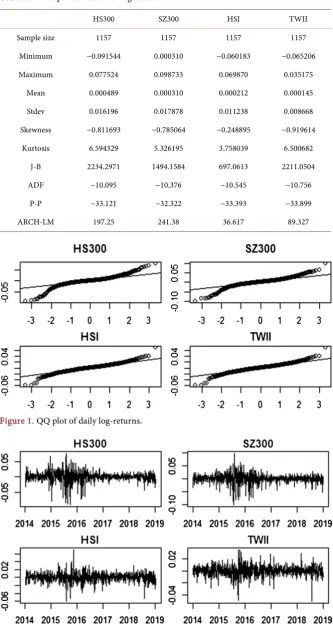
It can be seen from Table 1 that the daily logarithmic yield series of the Shanghai and Shenzhen 300 Index, the Shenzhen 300 Index, the Hang Seng Index and the Taiwan Weighted Index are all left-biased as the skewness is less than 0, and the kurtosis is significantly greater than 3, both with sharp peaks and thick tails feature. The J-B statistic rejects the null hypothesis of the normal distribution. It can also be seen from Figure 1 that the four indices are not obey to normal distribution as the scatter is away from the line. Both the ADF test and the P-P test passed, indicating that the yields of the four indices were stable. The volatility clustering feature refers to the fact that the volatility is high in a specific period of time while it is low in other periods. It can be seen from the daily logarithmic rate of return timing chart in Figure 2 that all four index yields exhibit volatility ag-gregation characteristics. The ARCH effect test is performed on the four yield series, and the results show that the rate of return series has conditional hete-roscedasticity.

3.2. GARCH Model Establishment

(6)

[image:6.595.207.541.80.714.2]

Table 1. Descriptive statistics of log-returns.

HS300 SZ300 HSI TWII

Sample size 1157 1157 1157 1157

Minimum −0.091544 0.000310 −0.060183 −0.065206

Maximum 0.077524 0.098733 0.069870 0.035175

Mean 0.000489 0.000310 0.000212 0.000145

Stdev 0.016196 0.017878 0.011238 0.008668

Skewness −0.811693 −0.785064 −0.248895 −0.919614

Kurtosis 6.594329 5.326195 3.758039 6.500682

J-B 2234.2971 1494.1584 697.0613 2211.0504

ADF −10.095 −10.376 −10.545 −10.756

P-P −33.121 −32.322 −33.393 −33.899

ARCH-LM 197.25 241.38 36.617 89.327

Figure 1. QQ plot of daily log-returns.

(7)

[image:7.595.207.540.553.637.2]

all stationary sequences, and all have an ARCH effect. The GARCH model not only reveals the “fluctuating aggregation” of financial markets, but also reveals the “thick tail” feature. According to previous scholars' research, the low-order GARCH (1, 1) model can well describe the characteristics of financial time series. Therefore, this paper establishes a low-order GARCH (1, 1) model for the Shanghai and Shenzhen 300 Index, the Shenzhen 300 Index, the Hang Seng Index and the Taiwan Weighted Index.

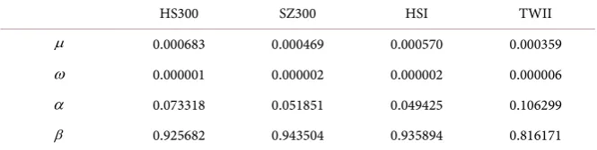
Table 2 is the parameter estimation results of the GARCH (1, 1) model, except for the constant term, all the parameters pass the significance test. Among them, the ARCH parameter α _{and the GARCH parameter}

β

are both greater than zero, which guarantees the positive definiteness of the conditional variance, and also indicates that fluctuations of the stock market are characterized by agglo-meration. The historical fluctuations are positively correlated with the current fluctuations and the speed is gradually slowed down. The large fluctuations often follow with large fluctuations, investors are more speculative in the stock market.

1

α β+ < ensure that the model is a smooth GARCH model.

A white noise test is performed on the standardized residual of the model, and the test statistic is the LB statistic. The results are shown in Table 3. Under the 6th

and 12th_{order lags, the P value of the LB statistic is significantly greater than 0.05.}

It can be considered that the residual of the model belongs to the white noise sequence, that is, the model can well characterize the log yield series.

3.3. POT Model Establishment

An estimate of the standard deviation can be obtained from the above GARCH (1, 1) model. Since the GARCH (1, 1) model measures the risks in the normal market, in reality, there are often a few extreme values that can cause huge losses. Therefore, here we establish a GARCH (1, 1)-POT model for the normalized re-sidual of the GARCH (1, 1) model, that is, model the super-threshold data ex-ceeding the threshold u. The most important thing to establish a POT model is the choice of threshold. If the threshold is too large, the sample data exceeding

Table 2. Parameter estimation of GARCH (1, 1) model.

µ _0.000683 _0.000469 _0.000570 _0.000359

ω 0.000001 0.000002 0.000002 0.000006

α 0.073318 0.051851 0.049425 0.106299

β _0.925682 _0.943504 _0.935894 _0.816171

Table 3. White noise test of residual.

(8)

the threshold will be too small, which may increase the variance of the parameter estimation. If the threshold is too small, the excess cannot be guaranteed to obey the generalized pareto distribution, which may result in biased parameter esti-mates. The method of selecting the threshold generally adopts the method of transcending the expectation function, and the selected threshold which value exceeds the threshold part to present a linear characteristic. In addition, there is the 10% principle proposed by Du Mouchel [12]: when the threshold u is allowed, about 10% of the data is selected as the extreme value data to be studied.

According to the graph of the transcendental expectation function of Figure 3, based on the 10% principle proposed by Du Mouchel, it can be seen that the mean excess plot shows a linear trend after 1.1 or 1.2. Therefore, the thresholds are se-lected to be 1.2, 1.2, 1.2 and 1.1 respectively. The generalized Pareto distribution (GPD) is fitted to the data exceeding the threshold, and the estimation results of the shape parameters and the scale parameters are shown in Table 4.

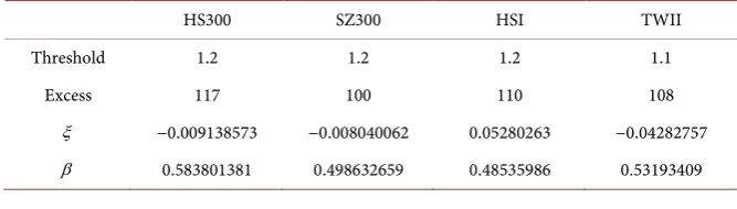
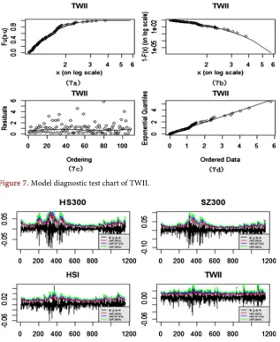
[image:8.595.208.540.419.597.2]

In order to test the fitting effect of the model, the diagnostic test charts of the GARCH (1, 1)-POT models of the standardized residuals of the four index yield series are shown in Figures 4-7 respectively. The upper left corner is the distri-bution function graph of the overrun, the upper right corner is the distridistri-bution tail probability estimation graph, the lower left corner is the residual scatter plot, and the lower right corner is the residual QQ plot. The closer the scatter and the line are, the better the model fits. It can be seen from the four graphs that most of the scatter points are on or near the line, and very few points have slight deviations

Figure 3. Mean excess plot.

Table 4. Model parameter estimation of GARCH (1,1)-POT model.

Threshold 1.2 1.2 1.2 1.1

Excess 117 100 110 108

ξ _{−0.009138573} _{−0.008040062} _0.05280263 _{−0.04282757}

[image:8.595.205.539.638.733.2]

(9)

[image:9.595.215.534.56.707.2]

Figure 4. Model diagnostic test chart of HS300.

[image:9.595.214.534.404.715.2]

Figure 5. Model diagnostic test chart of SZ300.

(10)

from the line, indicating that the effect of model is intended to be not bad, which also means that the threshold is reasonable.

3.4. VaR Calculation and Failure Rate Test

The VaR calculation is performed on the indices of the four stock markets. Figure 8 is a comparison between the index yields of the four stock markets and the VaR at the 0.05, 0.025, and 0.01 significance levels, showing the time-varying charac-teristics of the fluctuations. In particular, when the market rises or falls, the model will change the estimatimation of the next VaR at any time, reflecting the changes in the market in a timely manner. On the whole, most of the VaR values can fluctuate with fluctuations of the yield, and with the confidence level increases (that is, the level of significance decreases), the change is more close to the fluc-tuation of the yield. The part of the rate of return that fluctuates beyond VaR is a failure event. As the level of confidence increases, the number of failures decreases significantly.

[image:10.595.216.534.320.708.2]

The failure rate test is proposed by Kupiec [13]. The basic idea is to use the

Figure 7. Model diagnostic test chart of TWII.

(11)

model to calculate the predicted loss value and compare it with the actual loss value. When VaR is lower than the actual loss, it is recorded as a failure event. A successful event is recorded when VaR exceeds the actual loss. The actual failure rate is equal to the number of failure days N divided by the total number of ob-servations T, and the actual failure rate is compared with the significance level at which a given VaR estimate is achieved. The closer it is, the better the effect. The null hypothesis of the model is: H N T p0: = , where p is significant level. When

the actual failure rate is less than a given level of significance, the risk is overes-timated, and conversely, when the actual failure rate is greater than a given level of significance, the risk is underestimated.

If the actual failure rate is expressed as: L N 100%

T

= × _,

When N p

T < , the fitting success rate is: 100% 100%

L N

S

p Tp

= × = × _;

When N p

T > , the fitting success rate is: 100% 100%

p pT

S

L N

= × = × .

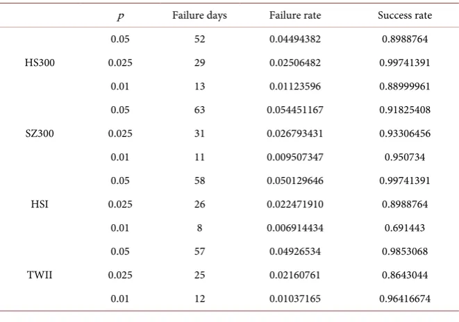
All in all, the fit success rate represents the ratio of the failure rate to the signi-ficance level of VaR. The signisigni-ficance level here is 0.05, 0.025 and 0.01, and Table 5 shows the results of the failure rate test.

[image:11.595.208.539.499.731.2]

From the results of the above failure rate test, the indices of the four stock markets have different degrees of overestimation and underestimation of risks. For the Shanghai and Shenzhen 300 Index, the risk is overestimated at a signi-ficance level of 0.05, while the risk is underestimated at a significant level of 0.025 and 0.01; for the Shenzhen 300, the risk is underestimated at a significant level of 0.05 and 0.025, while the risk is overestimated at a significance level of 0.01; for the Hang Seng Index, the risk is underestimated at a significance level of 0.05, while the risk is overestimated at a significant level of 0.025 and 0.01; for

Table 5. Failure rate test results.

p Failure days Failure rate Success rate

HS300

0.05 52 0.04494382 0.8988764

0.025 29 0.02506482 0.99741391

0.01 13 0.01123596 0.88999961

SZ300

0.05 63 0.054451167 0.91825408

0.025 31 0.026793431 0.93306456

0.01 11 0.009507347 0.950734

HSI

0.05 58 0.050129646 0.99741391

0.025 26 0.022471910 0.8988764

0.01 8 0.006914434 0.691443

TWII

0.05 57 0.04926534 0.9853068

0.025 25 0.02160761 0.8643044

(12)

a Taiwan Weighted Index, the risk is overestimated at a significant level of 0.05 and0.025, while the risk is underestimate at a significance level of 0.05. Among them, the Shanghai and Shenzhen 300 index has the highest success rate of the model under the significance level of 0.025 and the Hong Kong Hang Seng Index at the significance level of 0.05, and the Hang Seng Index has the lowest success rate at the significance level of 0.01. Overall, the model has a high success rate, which indicates that the combination of GARCH model and extreme value theory can measure the risk of Chinese stock market.

4. Conclusions

This paper analyzes the Shanghai and Shenzhen 300 Index of Shanghai stock exchange, Shenzhen 300 Index of Shenzhen stock exchange, Hang Seng Index of Hong Kong stock exchange market and Taiwan Weighted Index of Taiwan stock market, and combines GARCH model and extreme value theory to calculate separately. The VaR values of the Shanghai and Shenzhen 300 Index, the Shenzhen 300 Index, the Hang Seng Index and the Taiwan Weighted Index at the 0.05, 0.025 and 0.01 significance levels were calculated, and the failure rate was calculated, too. The GARCH model mainly depicts the “volatility aggregation” feature of financial time series. The GARCH-POT model adds the extreme value theory based on the extraction of the standard residual of GARCH model, which can well describe the influence of residual fluctuation of daily yield and reflect the "thick tail" of the distribution. Through empirical research and comparative analysis, the following conclusions are drawn:

The distribution of the yield of Chinese stock market has the characteristics of peak, thick tail and volatility. It is necessary to select the appropriate volatility model to fit the financial time series. The POT model with extreme value theory is added to the GARCH model to fit the tail portion of the yield. The failure rate test results show that the effect is better. However, regarding the selection of the thre-shold, it is somewhat subjective to rely solely on the observation of the graph beyond the expectation function. The methods such as the kurtosis method and the Hill estimation method are the future research directions. Since each stock market is not an independent entity, it conducts risk measurement on the stock market in mainland China, Hong Kong and Taiwan, studying its risk and its volatility spillover effect is very necessary for investors to construct diversified investment portfolios and relevant intra-regional formulation of departmental policies.

(13)

Fund

Project supported by the National Natural Science Foundation of China (61703117); National Natural Science Foundation of China (61763008); Guangxi Basic Ability Improvement Project of Young and Middle-aged Teachers (2018KY0261).

Conflicts of Interest

The authors declare no conflicts of interest regarding the publication of this pa-per.

References

[1] Wang, C.F. (2001) Financial Market Risk Management. Tianjin University Press, Tianjin.

[2] Engle, R.F. (1982) Autoregressive Conditional Heteroscedasticity with Estimates of the Variance of United Kingdom Inflation. Econometrica, 50, 987-1007.

https://doi.org/10.2307/1912773

[3] Bollerslev, T. and Bolleslev, T. (1986) Generalized Autoregressive Conditional He-teroskedasticity. Econometrica, 31, 307-327.

https://doi.org/10.1016/0304-4076(86)90063-1

[4] Nelson, D.B. (1991) Conditional Heteroskedasticity in Asset Returns: A New Ap-proach. Econometrica, 59, 347-370. https://doi.org/10.2307/2938260

[5] Gong, R., Chen, Z.C. and Yang, D.R. (2005) A Comparative Study and Comment on the Risk Value of Risks (VaR) in Chinese Stock Market by GARCH Model.

Quantitative and Technical Economic Research, 7, 67-81, 133.

[6] Dong, R., Zheng, H., Lu, Z.W. (2016) Recognition and Risk Measurement of Na-tional Debt Market Revenue Based on GARCH Family Model. Financial Theory and Practice, 1, 42-46.

[7] Mcneil, A.J. and Frey, R. (2000) Estimation of Tail-Related Risk Measures for Hete-roscedastic Financial Time Series: An Extreme Value Approach. Journal of Empiri-cal Finance, 7, 271-300. https://doi.org/10.1016/s0927-5398(00)00012-8

[8] Tang, Y. and Tang, Z.P. (2012) Research on Risk Value of Stock Market Based on POT Model. Southeast Academic, 4, 92-102.

[9] Zhang, H. and Wang, J. (2016) Risk Measurement of the Return Rate of Shanghai and Shenzhen Stock Markets Based on Extreme Value Perspective. Statistics & De-cision, 15, 163-165.

[10] Wang, M. and Wang, C.L. (2017) Exploring the Conditional Value of Risk Based on Return Volatility and Thick Tail—From the Examination of the Shanghai and Shenzhen 300 Index. Mathematics Practice and Theory, 47, 68-74.

[11] Pei, Y.H. and Yu, W.L. (2017) A Comparative Analysis of the Linkage between Shanghai and Hong Kong and Shanghai-US Stock Market before and after Shang-hai-Hong Kong Stock Connect. Wuhan Finance, 4, 26-29.

https://doi.org/10.2139/ssrn.3251660

[12] Du, M. and William, H. (1983) Estimating the Stable Index Alpha in Order to Measure Tail Thickness: A Critique. The Annals of Statistics, 11, 1019-1031. https://doi.org/10.1214/aos/1176346318