Decrease of the Penalty Parameter in Differentiable Penalty Function Methods

(1)

doi:10.4236/tel.2011.11003 Published Online May 2011 (http://www.SciRP.org/journal/tel)

Decrease of the Penalty Parameter in Differentiable

Penalty Function Methods

Roohollah Aliakbari Shandiz1, Emran Tohidi2

1

Faculty of Mathematical Sciences, Sharif University of Technology, Tehran, Iran

2

Department of Applied Mathematics, Ferdowsi University of Mashhad, Mashhad, Iran E-mail: [email protected], [email protected]

Received March 30, 2011; revised April 28, 2011; accepted May 4, 2011

Abstract

We propose a simple modification to the differentiable penalty methods for solving nonlinear programming problems. This modification decreases the penalty parameter and the ill-conditioning of the penalty method and leads to a faster convergence to the optimal solution. We extend the modification to the augmented La-grangian method and report some numerical results on several nonlinear programming test problems, show-ing the effectiveness of the proposed approach.

Keywords:Nonlinear Programming, Penalty Method, Penalty Parameter, Differentiable Penalty Methods

1. Introduction

Solving nonlinear programming (NLP) problems via a penalty method was first introduced by Courant [1] in 1943. Fiacco and McCormick [2] developed barrier methods for solving NLP problem. Murray [3] show that the Hessian matrix of penalty method is ill-conditioned. Since then, many approaches for reducing the ill-conditioning of penalty method were proposed. To avoid too increasing of the penalty parameter, Zangwill [4] introduced exact nondifferentiable penalty functions and Flet- cher [5] introduced continuously differentiable exact penalty functions. Another exact penalty methods have been studied in [6-13] and others. In addition, Mongeau [14] decreased the penalty parameter in exact penalty methods for solving linear programming problems. Here, Using general ideas of Mongeau, we propose an approach to reduce the penalty parameter in the differentiable penalty method for solving NLP problems.

2. The Basic Idea

Consider the following programming problem:





 

min

s.t. 0, = 1, , , ,

j

f x

NLP g x j m

x X

 



where f and the gj are twice continuously differen-

tiable functions.

Let > 0, a common penalty function for (NLP) is:

 

H1 H1

 

x =f

 

x P x

 

,

 __

where,

 

= m₌₁ _j

 

2

j

P x



g x and

 

= max 0,



 



j j

g x g x .

A penalty problem for (NLP) is defined as follows:





min 1

 

=

 

1

s.t. .

H x f x P x

PEN

x X

 __

 Gradient and hessian of H1



can be calculated as follows:

 

1

=1 =

= 2 ,

m

j j

j

H x f x P x

f x g x g x

 _

 

   

 





 

2 2 2

1

2 2

=1

=1 =

= 2

2 .

m

j j

j

m

T

j j

j

H x f x P x

f x g x g x

g x g x

 _





 

   

  

  



Let

 

= 2 m₌₁ _j

 

2 _j

 

j

U x



g x  g x and

 

= 2 =1

 

m T

j j

j

(2)

 

2 2

1 = .

H x f x U x V x

    (2.1)

Note that due to the continuity of second derivatives, Hessian matrices 2f , 2P and 2gj are sym-

metric.

The condition number of a square matrix A is given by K

 

A = A A1 . If K A

 

is large, then A is said to be ill-conditioned. For a symmetric matrix A, it can be shown that

 

= max min,

K A  

where, max and min are the largest and smallest

eigenvalues of matrix A, respectively.

If we assume that there are r active constraints at

*

x , the optimal solution of (NLP), and The gradients of these constraints are linearly independent, Then V has rank equal to r and thus has r nonzero eigenvalues. (2.1) implies that when   at least r eigenvalues of 2

1

H

 tend to infinity. It has been shown in [15] that exactly r eigenvalues tend to infinity and n r other eigenvalues tend to finite limits, which implies the ill- conditioning of the Hessian of penalty method.

To avoid the ill-conditioning, instead of usual penalty function we consider the following function:



H2



H2

 

x =f

 

x P x

 

, > 0.

 __ _

Its corresponding penalty problem for (NLP) is:





min 2

 

=

 

2

s.t. .

H x f x P x

PEN

x X

 _{ }



It is easy to see that problems (PEN1) and (PEN2) are equivalent. Because H1

 

x = H2

 

x

 _ 

. Gradient and Hessian of H2



is

 

2 = ,

H x f x  P x

   

 

2 2 2

2

2 =

= .

H x f x P x

f x U x V x

 _



   

  

If 2

 

*

P x

 is of full rank (for example, if P is a strict- ly convex function), then all eigenvalues of 2

 

*

P x 

are nonzero. Thus, for a large enough  all eigenvalues of 2

 

*

2

H x

 are also nonzero. Therefore un- like H1



, H2



is not ill-conditioned. Consider the following example.

Example 1. Consider

 

2

min = 1

s.t. 1 = 0.

f x x

x

 

The optimal solution is x*= 1. We have:

 

2





2

1 = 1 1 ,

H x x   x

 





1 = 2 2 1 ,

H x x  x

  

 

2

1 = 2 2 ,

H x 

 

and

 



2







2

2 = 1 1 ,

H x x   x

 





2 = 2 2 1 ,

H x x  x

  

 

2

2 = 2 2.

H x 

 

Therefore when  , the hessian matrix 2H1





tends to infinity, But 2H2



 tends to a fixed number. Although under some assumption the hessian of

2 2

H

 is not ill-conditioned but there is a problem. For every feasible point

x

we have P x

 

= 0, and for too large , the value of f x

 

 is very close to zero. Thus, near the boundary of feasible region,

 





2 =

H f x  P x

   is almost zero and this cause the termination of the penalty method. So the penalty method with H2



only gives a feasible point and does not converge to optimal solution or converges very slowly.

Thus, to have advantages of both H1



and H2



, we consider the following combined formula:

 

3 = .

H x f x   P x

This penalty function apply penalty two times, once by multiplying P x

 

by  and again by dividing f x

 

by  . In fact, H3



is equivalent to the following penalty function in which a  has been factorized:

 

2

 

4 = .

H x f x  P x But order of 2H3



 is O

 

 while order of 2H4





is O

 

2 . This leads to faster convergence of penalty method using H3



than that using H4



.

We use the following general formula instead of H3



:

 

= f x

_{ }

 

,

H x P x

  

where, :   is a positive and increasing function in terms of .

Lemma 2.1 Consider the following problem:





min

 

=

 

s.t. .

f x

H x P x

PEN

x X

 _

  



Suppose that for each > 0 there exists a solution xX for (PEN), and that x is obtained in a com- pact subsets of X. Then, any limit point of x is a solution to (NLP).

Proof. Consider the following problem:

 

   

min

s.t. ,

f x P x

x X

(3)

Since f x

 

 

   

P x = 

 

H

 

x , clearly the problem is equivalent to (PEN). Since  

 

  when  , thus considering  

 

as a penalty parameter and applying Theorem 9.2.2 of [6] implies the result.

Although 2H1



 and 2H are both of O

 

 order, but H1



is a penalty function with penalty parameter  and H is equivalent to a penalty function with penalty parameter  

 

(see proof of Lemma 2.1). Since for larger penalty parameter solution of penalty problem is closer to the solution of main problem, largeness of  

 

in comparison with  leads to faster convergence of the penalty method.

3. Extension to Augmented Lagrangian

Methods

The augmented Lagrangian for Problem (NLP) is defined as follows:





 

2

1

=1 =1

, =

m m

j j j

j j

A x f x 



 G 



G

where = max

 

, 2

j

j j

G g x 



 



 

 .

It has been shown that if *

is the Lagrange mul- tiplier of (NLP) at the optimal solution _x*

Then for large enough , minimization of



*



1 ,

A x gives the optimal solution of (NLP). Thus, A1



is said to be exact for solving (NLP).

Since at first the value of *

is not often available, the following formula is usually used for updating the values of _j:

1₌ ₂ _{, = 1, 2,} _,

k k k

j j kGj j m



   _  _

Now consider A1  



x,



  _

. We can write it as follows:  

_

_

 



 



1 2 =1 =1 , = p

j j _m

j

j j

A x

f x G

G                    _       



Thus, from the discussion of previous section, instead of A1



we consider the following penalty function:





 



 



2 =1 =1 , = p

j j _m

j

j j

f x G

A x G

           



Since the ordinary augmented Lagrangian method for solving (NLP) is exact and we also have





_{ }

 

1 1

, = ,

A x A 

  (3.1) clearly similar to the ordinary augmented Lagrangian method we have the following result.

Lemma 3.1 Suppose that second order sufficient conditions for (NLP) are satisfied at x*, *. Then there exists a 0 such that for any  > 0,

*

x is a local minimizer of _A



_x_,*



.

From (3.1), we can consider A as an ordinary augmented lagrangian with penalty parameter  

 

. Thus, new updating formula for the j is as follows:

 

1

= 2 , = 1, 2, ,

k k k k

j j k k Gj j m

  

   _    _

4. Computational Results

4.1. Algorithms

Consider the following augmented Lagrangian problem for (NLP):

 





 



 



2 =1 =1

min , =

s.t. .

p j

j j _m

j j

j j j

f x G

A x G

PA x X              



where,  is the average of the j. For solving (NLP)

via augmented Lagrangian method we apply the following algorithm where is similar to Algorithm 1 of [11] with the first order update rule of Lagrangian multipliers.

Algorithm 1

Define

 

1 

 

T 1

= , , m

m

G x _G   x  G   x _ . {Given: 0 0

,

x  }

0

xx

0



2, = 1, ,

j j m

  

 

viol G x _

while _iol_{> 10}8

{line search method for solving (PA)} counter0

while _xA > 1016 and





< 3 1 counter m n 

dN  modified BFGS direction

(4)

x x dN

countercounter1

end(while) viol G x

 





if viol< 1 / 4viol

 

2 j , = 1, ,

j j j Gj j m

  

      

end(if)

for j= 1,,m

if j 

 

> 1 / 4

j

G   x viol

 





1.3

 

j j

       end(if)

end(for)

if viol< 1 / 4viol violviol end(if)

end(while)

For solving (NLP) via the penalty method, we refine Algorithm 1 by considering  as zero and removing the step of its updating. Also, we solve the following problem in line search method of the algorithm:

 

_{ }

 

2 =1

min =

s.t. .

m

j j j

f x

H x g x

x X

  



 



4.2. Test Results

Algorithms 1 is programmed in MATLAB 7.6 and run on a PC with 1.8 GHz and 1 GB RAM. For solving subproblems we use a line search algorithm. The step length is determined by the Goldstein test and the direction is determined by the BFGS formula with Powell’s modifications [16] (the eigenvalues are considered as zero). The function  is considered as

 

= 

   for = 0, , ,1,1.5, 2, 41 1 4 2

 . For each test problem we take a fixed initial point.

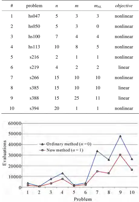
All the test problems with one or more constraints are selected from Hock and Schittkowski’s set [17] and Schittkowski’'s set [18] located in [19]. The characteristics of test problems are listed in Table 1, where n is the number of variables, m the total number of constraints, mNL the number of nonlinear constraints

and objective the type of the objective function (linear/ nonlinear).

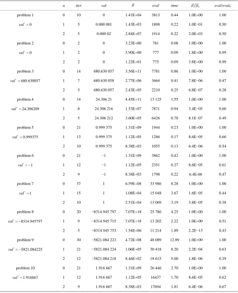
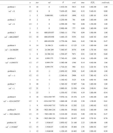
The computational results for the penalty method and the augmented Lagrangian method are summarized in Tables 2 and 3, respectively. The following symbols are used in these tables:

val* = optimal value of the test problem. val = the obtained optimal value.

iter= number of iterations.

eval = number of function evaluations.

eval0 = eval for the ordinary penalty method ( = 0)

 = the average of j, = 1,j ,m when the algorithm terminates.

0

  in case  = 0.

[image:4.595.307.537.188.523.2]

time: CPU time (seconds) to reach the solution.

Table 1. Problem characteristics for test problems.

# problem n m mNL objective

1 hs047 5 3 3 nonlinear

5 s216 2 1 1 nonlinear

6 s219 4 2 2 linear

8 s385 15 10 10 linear

9 s388 15 25 11 linear

[image:4.595.306.539.188.524.2]

Figure 1. Comparison of ordinary penalty method (α = 0) and new penalty method (α = 1).

[image:4.595.310.538.561.693.2]

(5)

[image:5.595.70.539.95.672.2]

Table 2. Numerical results for the ordinary penalty method (α = 0) and the new penalty method (α = 1, 2).

α iter val  eval time  0 eval/eval0

problem 1 0 10 0 1.41E+04 3813 0.44 1.0E+00 1.00

*

= 0

val 1 5 0.000 001 1.43E+03 1898 0.22 1.0E−01 0.50

2 5 0.000 02 2.84E+07 1914 0.22 2.0E+03 0.50

problem 2 0 2 0 3.23E+00 781 0.08 1.0E+00 1.00

*

= 0

val 1 2 0 5.90E+00 777 0.09 1.8E+00 0.99

2 2 0 1.22E+01 775 0.09 3.8E+00 0.99

problem 3 0 14 680.630 057 3.56E+11 7781 0.86 1.0E+00 1.00

*

= 680.630057

val 1 7 680.630 058 2.77E+06 3664 0.41 7.8E−06 0.47

2 5 680.630 057 2.43E+05 2210 0.25 6.8E−07 0.28

problem 4 0 14 24.306 21 4.45E+11 13 125 1.55 1.0E+00 1.00

*

= 24.306209

val 1 8 24.306 216 1.53E+07 7871 0.94 3.4E−05 0.60

2 5 24.306 212 3.60E+05 6426 0.78 8.1E−07 0.49

problem 5 0 21 0.999 375 1.31E+09 1944 0.23 1.0E+00 1.00

*

= 0.999375

val 1 13 0.999 375 1.12E+05 1286 0.17 8.6E−05 0.66

2 10 0.999 375 8.38E+03 1055 0.13 6.4E−06 0.54

problem 6 0 21 −1 1.31E+09 3862 0.42 1.0E+00 1.00

*

= 1

val  1 12 −1 1.12E+05 2351 0.27 8.6E−05 0.61

2 9 −1 8.38E+03 1798 0.22 6.4E-06 0.47

problem 7 0 37 1 6.59E+08 33 986 8.28 1.0E+00 1.00

*

= 1

val 1 15 1 1.08E+04 15 048 3.67 1.6E−05 0.44

2 10 1 2.51E+04 13 069 3.19 3.8E−05 0.38

problem 8 0 20 −8314.945 797 7.07E+18 25 786 4.25 1.0E+00 1.00

*

= 8314.945797

val  1 9 −8314.945 715 7.07E+18 13 202 2.22 1.0E+00 0.51

2 5 −8314.945 753 1.54E+06 11 214 1.89 2.2E−13 0.43

problem 9 0 30 −5821.084 223 4.72E+08 48 089 12.89 1.0E+00 1.00

*

= 5821.084225

val  1 21 −5821.084 224 1.06E+05 30 418 8.20 2.2E−04 0.63

2 12 −5821.084 218 8.46E+02 18 615 5.00 1.8E−06 0.39

problem 10 0 21 1.916 667 1.31E+09 26 446 2.70 1.0E+00 1.00

*

= 1.916667

val 1 12 1.916 667 1.12E+05 16437 1.70 8.6E−05 0.62

2 9 1.916 667 8.38E+03 17694 1.81 6.4E−06 0.67

Note that tables rows corresponding to  = 0 show numerical results for the ordinary methods and other rows show numerical results for the new methods.

(6)

[image:6.595.71.540.95.649.2]

Table 3. Numerical results for the ordinary penalty method (α = 0) and the new penalty method (α = 1/2, 1).

α iter val  eval time  0 eval/eval0

problem 1 0 10 0 1.41E+04 3813 0.42 1.0E+00 1.00

*

= 0

val 1/2 8 0 7.63E+05 3041 0.33 5.4E+01 0.80

1 5 0.000 001 1.43E+03 1898 0.22 1.0E−01 0.50

problem 2 0 2 0 3.23E+00 781 0.08 1.0E+00 1.00

*

= 0

val 1/2 2 0 4.29E+00 783 0.08 1.3E+00 1.00

1 2 0 5.90E+00 777 0.09 1.8E+00 0.99

problem 3 0 14 680.630 057 3.56E+11 7781 0.89 1.0E+00 1.00

*

= 680.630057

val 1/2 10 680.630 058 1.64E+10 5355 0.61 4.6E−02 0.69

1 7 680.630 058 2.77E+06 3664 0.42 7.8E−06 0.47

problem 4 0 14 24.306 21 4.45E+11 13 125 1.55 1.0E+00 1.00

*

= 24.306209

val 1/2 9 24.306 209 7.36E+07 8376 0.98 1.7E−04 0.64

1 8 24.306 216 1.53E+07 7871 0.91 3.4E−05 0.60

problem 5 0 14 0.999 375 7.74E+01 1269 0.16 1.0E+00 1.00

*

= 0.999375

val 1/2 17 0.999 379 3.38E+08 1346 0.14 4.4E+06 1.06

1 11 0.999 375 1.71E+01 994 0.11 2.2E−01 0.78

problem 6 0 19 −1 2.85E+02 3928 0.45 1.0E+00 1.00

*

= 1

val  1/2 13 −1 2.24E+01 2908 0.33 7.8E−02 0.74

1 14 −1 1.14E+02 3125 0.36 4.0E−01 0.80

problem 7 0 40 1 1.34E+02 32 887 7.66 1.0E+00 1.00

*

= 1

val 1/2 21 1 3.88E+01 21 026 4.94 2.9E-01 0.64

1 22 1 1.33E+02 17 851 4.19 1.0E+00 0.54

problem 8 0 18 −8314.945 797 7.07E+16 25 476 4.19 1.0E+00 1.00

*

= 8314.945797

val  1/2 9 −8314.945 793 1.06E+08 15 430 2.58 1.5E-09 0.61

1 9 −8314.945 715 7.07E+18 13 202 2.22 1.0E+02 0.52

problem 9 0 36 −5821.084 218 1.10E+04 39 826 10.52 1.0E+00 1.00

*

= 5821.084225

val  1/2 15 −5821.084 18 3.21E+00 18 624 5.00 2.9E−04 0.47

1 26 −5821.084 224 2.93E+03 30 457 8.03 2.7E−01 0.76

problem 10 0 17 1.9166 67 2.85E+02 21 168 2.23 1.0E+00 1.00

*

= 1.916667

val 1/2 15 1.9166 67 1.14E+04 18 404 1.91 4.0E+01 0.87

1 12 1.9168 88 1.12E+05 10 483 1.09 3.9E+02 0.50

thods decrease number of iterations and number of function evaluations and as we expect the penalty method notably reduce the penalty parameter.

We observed in computational results that although for larger  the convergence is faster, for some test

(7)

of feasible region. Thus, we suggest use of  such that 1. That is, use of the  with the order greater than O

 

 is not recommended. Here, for having more efficiency we suggest  

 

= for the penalty method and  

 

=  for the augmented Lagrangian method.

In Figure 1 number of function evaluations for the ordinary penalty method ( = 0) and new penalty method ( = 1) is compared. The comparison of evaluations of ordinary augmented Lagrangian (= 0) and new augmented Lagrangian ( = 1 2) is illustrated in Figure 2.

5. Conclusions

We proposed a simple modification to the penalty methods and showed that the new penalty methods has better performance than the usual penalty methods. Computational results on several test problems showed that number of iterations decreases and calculations significantly reduce.

6. References

[1] R. Courant, “Variational Methods for the Solution of Problems of Equilibrium and Vibrations,” Bulletin of the American Mathematical Sociaty, Vol. 49, No. 1, 1943, pp.

1-23.

[2] A. V. Fiacco and G. P. McCormick, “Nonlinear Pro-gramming: Sequential Unconstrained Minimization Tech- niques,” Society for Industrial and Applied Mathematics, McLean, 1990.

[3] D. M. Murray and S. J. Yakowitz, “Constrained Differen-tial Dynamic Programming and Its Application to Mul-tireservior Control,” Water Resources Research, Vol. 15, No. 5, 1979, pp. 1017-1027.

[4] W. I. Zangwill, “Nonlinear Programming via Penalty Functions,” Management Science, Vol. 13, No. 5, 1967, pp. 344-358.

[5] R. Fletcher, “A Class of Methods for Nonlinear Pro-gramming with Termination and Convergence Proper-ties,” Integer and Nonlinear Programming, Amsterdam, 1970, pp. 157-173.

[6] M. S. Bazaraa, H. D. Sherali and C. M. Shetty, “Nonlin-ear Programming: Theory and Algorithms,” 3rd Edition, Wiley, New York, 2006.

[7] C. Charalambous, “A Lower Bound for the Controlling

Parameters of the Exact Penalty Functions,” Mathemati-cal Programming, Vol. 15, No. 1, 1978, pp. 278-290.

[8] A. R. Conn, “Constrained Optimization Using a Nondif-ferentiable Penalty Function,” SIAM Journal of Numeri-cal Analysis, Vol. 10, No. 4, 1973, pp. 760-784.

[9] G. D. Pillo and L. Grippo, “A Continuously Differenti-able Exact Penalty Function for Nonlinear Programming Problems with Inequality Constraints,” SIAM Journal of Control and Optimization, Vol. 23, No. 1, 1985, pp. 72-

84.

[10] G. D. Pillo and L. Grippo, “Exact Penalty Functions in Constrained Optimization,” SIAM Journal of Control and Optimization, Vol. 27, No. 6, 1989, pp. 1333-1360.

[11] J.-P. Dussault, “Improved Convergence Order for Aug-mented Penalty Algorithms,” Computational Optimiza-tion and ApplicaOptimiza-tions, Vol. 44, No. 3, 2009, pp. 373-383.

[12] A. L. Peressini, F. E. Sullivan and J. J. Uhl, “The Ma-thematics of Nonlinear Programming,” Springer-Verlag, New York, 1988.

[13] T. Pietrzykowski, “An Exact Potential Method for Con-strained Maxima,” SIAM Journal of Numerical Analysis, Vol. 6, No. 2, 1969, pp. 294-304. [14] M. Mongeau and A. Sartenaer, “Automatic Decrease of

the Penalty Parameterin Exact Penalty Function Meth-ods,” European Journal of Operational Research, Vol. 83, No. 3, 1995, pp. 686-699.

[15] D. G. Luenberger and Y. Ye, “Linear and Nonlinear Pro-gramming,” 3rd Edition, Springer, New York, 2008. [16] M. J. D. Powell, “A Fast Algorithm for Nonlinearly

Con-strained Optimization Calculations,” Lecture Notes in Mathematics, Vol. 630, 1978, pp. 144-157.

[17] W. Hock and K. Schittkowski, “Test Examples for Non-linear Programming Codes,” Journal of Optimization Theory and Applications, Vol. 30, No. 1, 1980, pp. 127- 129.

[18] K. Schittkowski, “More Test Examples for Nonlinear Programming Codes (Lecture Notes in Economics and Mathematical Systems),” Springer, Berlin, 1987.

[19] Princeton Library of Nonlinear Programming Models, 2011.