5) To open a new model file, click on the new model icon as shown on the next page, or click on File

1

ECE-205 Lab 1

Introduction to Simulink and Matlab

Throughout this lab we will focus on determining the behavior of a first order system written in the standard form

( ( )

(

) )

y dy t

dt t Kx t

τ + =

wherex t( )is the input, y t( )is the output, τ is the time constant, and K is the static gain. We will first introduce Simulink for modeling this system, then show how we can use Matlab to run the Simulink file, and finally how we can use Matlab to produce some nice plots and do some other cool stuff. For the most part, just following along and type what you are told to type. You will only learn by doing (and seeing examples). The following examples will be specific to Matlab 2012b, but you can use them with only minor modifications for other versions of Matlab. The only thing you need to include in your memo is at the end of the lab, but you will need to work through the rest of the lab to get there.

PART I

1) In order to make our simulation diagram, we need to solve for the highest derivative power,

( ) ( ) ( )

y t Kx t y t

τ = −

or

y t( ) 1

[

]

= −



Clearly if we integrate y t( ) we will gety t( ). So our simulation diagram will require some scaling (or gain blocks), a summing block, and an integration block.

2) Next you need to create a folder for Matlab to store the files you will be generating in. Although Matlab has a default folder, it is much better practice to have individual folders for each class (or lab, etc). So create a folder for Matlab.

2 4) Since we are going to use Simulink first, open the Simulink Library by clicking on the icon at the stop of the Matlab command window, or type simulink (all lower case) in the command window (and hit enter).

A window will pop up that looks something like that on the following page.

5) To open a new model file, click on the new model icon as shown on the next page, or click on File, select New, then select Model.

Yet another window will open up for you, and this is where you will build your Simulink model. In order to save your work, in this new window click on File, then Save As, then you need to give it a name with the suffix slx. Let’s assume you name your model file test.slx.

Click here to change folders

This is probably the default folder location, but it is a bad folder location

3

Before we go on, let’s set some parameters. Let’s assume τ =0.02seconds, K =0.5, and the input is a step with amplitude A=0.5. Now we will build our model.

6) In the Simulink Library Browser, scroll down until you see a block named Sources as shown in the above figure, and then double click on it. This is where we will find our available system inputs.

7) Drag Clock over to your Simulink model file, test.slx, and then scroll down to find Step and drag this over to your model file.

Click on this icon to open a new model file.

4 8) Next we are going to need a Sink, or a way to save or plot our results. In the left panel, click on

Sinks as shown below and then drag XY graph over to test.slx. Be sure to save test.slx regularly so you do not lose your work.

9) We are going to need an integrator, so click on Commonly Used Blocks in the left panel, and drag an

Integrator (1/s) over to your model file, drag a Sum over to your model file, and then drag a Gain over to your model file.

5

At this point, you have a pretty random set of blocks in your test.slx file, and we need to start

connecting them. Most often people think of their simulations going from left to right, so that is how we will set ours up. Be sure to save test.slx now, and regularly!

10) Rearrange the blocks in the general order you will use them, as shown in the following figure. At this point you probably realize you will need another Gain block. You can go back to the Library Browser, or just right click on the Gain block you have and choose copy and then paste.

11) Now we are ready to connect our blocks. This takes some practice, but you generally click on the source or destination block (you will figure out what works for you). Connect the blocks so your file looks like the next figure. To get the bottom line into the summer, you may want to make a line going down from the sum block, let go, then make a separate line from your first line to the line after the

integrator. Keep in mind that we are trying to solve the equation y t( ) 1

[

]

= −

 , so try to follow

6

Next we need to clean some things up and start entering our parameters.

12) Double click on the Step block, and set the Step Time to 0 and the Final Value ( the amplitude of the step) to 0.5 (the value of A). Then click OK.

13) Double click on the Gain block next to the Step block, and set the gain equal to 0.5 (the value of K), and then click OK.

14) Double Click on the Sum block. We will change the parameters, as shown in the figure. Let’s choose a rectangular sum block (this works better if there are more inputs), and change the bottom sign to -, which is what we want. Also, we will put in extra space by adding some space, denoted by |. After you click OK you will see the change in the Sum block in your model file. The changes are shown on the next page.

15) The next Gain block represents 1 /τ, so double click on it and enter 50, then click OK.

16) We want to be able to see our output, so double click on the XY Graph and enter x-min = 0, x-max = 0.3, y-x-min = 0, y-max = 0.3, then click OK.

x Kx dy/dt

7 17) If we are only going to plot our output from 0 to 0.3 seconds, there is no reason to run the

simulation any longer than this. Change the final time of the simulation to 0.3, and then run the simulation by pressing the play button, as shown on the following figure.

If you have done everything correctly, you should get a graph like the following:

8 PART II

While the XY Graph is nice for getting a basic idea of what is going on, you have little control over how the graph is presented. You also need to know a lot about the signal you want plotted. Matlab, however, has some very nice graphing capabilities, so we would like to be able to use them. What we need is a way to access the data we have generated.

1) Go back to the Simulink Library Browser, click on Sinks, and then drag two simout (To Workspace) blocks over to your simulating file (test.slx).

2) Right click on XY graph to delete it. You can click on data paths to delete them also.

3) Connect the simulation output (y) and the clock to the two different simout blocks, as shown in the following figure. (It will rename one of the simout blocks simout1, but we will change the names in a bit.)

4) Double click on the simout block connected to the clock. Set the Variable name to time and the Save format to Array.

5) Double click on the simuout block connected the integrator. Set the Variable name to y and the

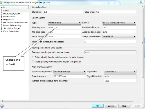
9 6) Run the simulation. It will not appear that anything much has happened, but you will likely get some warning messages in the Matlab command window about a default step size. We can just let Simulink use the default step size, but sometimes it is better to set it ourselves. In the model window, click on

Simulation and select Model Configuration Parameters. You should get a window like the following figure. For now, set the Max step size to 1e-6 and click on ok. Save your model file and run it again. You should no longer get any complaints about the step size. However, you still do not have any figures plotted either! T he simulation has saved the data to your workspace. Type who in the Matlab command window, and you should see that both time and y (and maybe some other variables) are now in the workspace.

7) To plot the results of the simulation, type the following lines into the Matlab command window,

plot(time,y); grid; xlabel('Time (sec)'); ylabel('y(t)'); title('First Order System');

and you should get a graph like that shown on the next page.

10 PART III

Just as in general programming it is a bad thing to “hard code” a variable, the same is true with Simulink. For example, we would like to be able to change the parameters in our simulation, run the simulation, and plot the results in a very convenient way. This is what we will accomplish in this level.

1) In the Matlab command window, select New Script (at the top left of the window) Yet another new window will open up!

2) In this new window, select Save, then Save As, and then name it test_driver.m.

3) In this new file, type the following lines: %

% clear all variables %

clear variables

%

% this program runs the file test.mdl %

sim('test.mdl');

Any line in Matlab that begins with a % is a comment line. The line sim(‘test.slx’); actually runs the Simulink file.

4) Save this file, then run it, as shown in the figure below:

0 0.05 0.1 0.15 0.2 0.25 0.3 0.35

0 0.05 0.1 0.15 0.2 0.25

Time (sec)

y

(t

)

11 5) To see that this is working, in the Matlab workspace type clear, then who. There should be no

variables in the workspace. The run your file test_driver.m and type who in the workspace, and you should see variables have been generated.

6) We would also like to automatically generate a plot everytime we run our Matlab program, so enter the following lines into your Matlab program (after the sim command, so the data is in the workspace)

plot(time,y); grid; xlabel('Time (sec)'); ylabel('y(t)');

title('First Order System');

You should run (play) the program again, and if should generate a graph (figure) like before. You may want to remove any figures before you run it to be sure it generated a new figure.

7) If may also be useful for use to plot both the output (y t( )) and the steady state valueKA. To do this, first modify your Simulink file test.slx to look like the following figure. You may need to select an entire group of elements in Simulink to shift your elements around.

12 8) Modify the plotting commands in your Matlab file test_driver.m as follows:

plot(time,y, 'b- ',time,Kx,'r--'); legend('y(t) ', 'y_{ss}'); grid; axis([ 0 max(time) 0 max(y)*1.1]);

xlabel('Time (sec)'); ylabel('y(t)');

title('First Order System');

Matlab defaults to finding a convenient set of axes, but sometimes you want to tell Matlab more specifically the axes you want. If you type help plot in the Matlab command window you can find a number of options for plotting. If you run your code now, you should get a figure like the following. Note that you can drag the Legend around and put it where ever you want.

0 0.05 0.1 0.15 0.2 0.25 0.3

0 0.05 0.1 0.15 0.2 0.25

Time(sec)

y

(t

)

First Order System

13 9) Finally, we would like all of the parameters we have in our Simulink model file to be controlled by the Matlab program. Modify the Matlab program test_driver.m and put the following lines before the simulation command (sim)

tau = 0.02; K = 0.5; A = 0.5; Tf = 0.3;

Next, edit the Simulink file, and use these variable names instead of the values you entered previously. The final value of the step should now be A, the gain of the first gain block should be K, and the gain of the second gain block should be 1/tau. The final time of the simulation should be changed to Tf.. Delete any figures and run your Matlab driver file again. You should get the same figure as before.

PART IV

As long as we are putting all of the variables in our Matlab file (program), we might as well figure out how we can use this to generate an input.

1) Go to the Simulink Library Browser, click on Sources, and drag a simin (From Workspace) block over to your Simulink model file. Delete the Step block and connect this block as the input.

2) Double click on the simin block and name the Data xt. This is where Simulink will look for its input data. Note that you will need to produce both data values (x t( )) and time values (t) and put them into the variable xt. We will show you one way to do this next. Also, Simulink will interpolate between the data values as it needs to.

3) Now we need to generate some data and put it into the correct format. We will use what Matlab calls an anonymous function to do this. We will generate the following signal

0.1 0. 1 0 ( ) 1 1 t x t t = − ≤ <   _≥ 

To do this type the following lines in your Matlab code before the sim command and after you have defined Tf:

%

% generate the input %

x = @(t) 1*((t>=0)&(t<0.1)) -1*(t>=0.1); t = linspace(0,Tf,300);

14

The first piece of code after the comment is the definition of x t( ). The second line of code tells Matlab

to generate an array of time values for 0 to Tf, and use 300 evenly spaced points. The third line of code puts the data in the correct form for Simulink. The apostrophe means to take the transpose, the brackets [] mean form an array, and x(t) tells Matlab to evaluate the function x at the specified times t. (Note that you might feel that it would be easier to use Matlab’s heaviside function here, but sometimes Simulink complains, since Matlab defined the heaviside function evaluated at zero to be not a number (NAN).) Comment out the axis command and run your code, you should get a graph like the following:

4) Now let’s try something more complicated. In the notes we have an example for a first order system with parameters τ =0.0001, K =0.01, and the initial conditiony(0)=0.01. The system input is

0 0

2 0 0.0001

( )

3 0.0001 0.00025

4 0.00025 t t x t t t < 

 _{≤ <}



= _{− ≤ <}



 _≥



Change all of the parameters in your Matlab file to match these, and set the simulation final time to 0.0008 seconds. Make a new variable called y0, and set y0 = 0.01; Click on the integrator in your Simulink file and set the Initial condition to y0.

0 0.05 0.1 0.15 0.2 0.25 0.3 0.35

-0.5 -0.4 -0.3 -0.2 -0.1 0 0.1 0.2 0.3 0.4 0.5 Time (sec) y (t )

First Order System

15

To enter the input, change the definition of the function as follows:

x = @(t) 0*(t<0)+2*((t>=0)&(t<0.0001))...

-3*((t>=0.0001)&(t<0.00025))+4*(t>=0.00025);

Note that to continue a Matlab function or statement on the next line, you end the line with three dots (…)

If you have done everything correctly, comment out the axis command, and run the code, you should get the following graph:

PART V

Finally, when you are doing your homework, you are going to have problems like these, and are going to want to know how to check your answers. Now that we know how to use anonymous functions and Matlab, we can check our answers. For this problem, the solution is

/0.0001

( 0.0001)/0.0001

( 0.00025)/0.0001

0 0

0.01 0.02 0 0.0001

( )

0.04632 0.03 0.0001 0.00025

0.05966 0.04 0.00025

t t t t e t y t e t e t − − − − − < 

 _{− + ≤ <}



=  _{− ≤ <}



− + ≥



0 1 2 3 4 5 6 7 8

x 10-4 -0.03 -0.02 -0.01 0 0.01 0.02 0.03 0.04 Time(sec) y (t )

First Order System

y(t) y

16

In Matlab, type in the following anonymous function just below your definition of your anonymous definition for x,

ya = @(t) 0*(t<0)+(-0.01*exp(-t/0.0001)+0.02).*((t>=0)&(t<0.0001)) ...

+(0.04632*exp(-(t-0.0001)/0.0001)-0.03).*((t>=0.0001)&(t<0.00025))... +(-0.05966*exp(-(t-0.00025)/0.0001)+0.04).*(t >=0.00025);

Next change your plotting and legend commands to the following:

plot(time,y,'b-',time,Kx,'r--',time,ya(time),'mo'); legend('y(t)','y_{ss}','y_{analytical}');

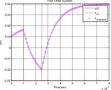
If your everything work correctly, you should get the following plot, which shows the analytical solution matches the simulated solution.

In this figure, it is difficult to really see the difference between the analytical and Simulink solutions. This is because we are using so many data points. One of the ways to get around this is to downsample the time. Let’s define a new variable (before the print command and after we have run the simulation)

0 1 2 3 4 5 6 7 8

x 10-4 -0.03

-0.02 -0.01 0 0.01 0.02 0.03 0.04

Time(sec)

y

(t

)

First Order System

y(t) y

ss y

17 td = downsample(time, 10);

This says, loosely speaking, that the variable td will be approximately every 10th data point in the array time. We now want to change the plot command to the following:

plot(time,y,'b-',time,Kx,'r--',td,ya(td),'mo');

This should produce the following plot.

At this point, you need to email me a memo which includes your version of the above graph. Your memo must be formatted in a reasonable memo format (to, from, date, etc.) and be a word document (do not just send an e-mail with the memo as a body). To include this graph, in the window in which your figure appears select Edit and then Copy Figure. You can then past the figure in your memo. Do not include your figure using any other method! Be sure the figure is large enough I can see it and that it has a figure number and caption. If you have any comments or suggestions for improving this lab, please add them to your memo, but they are not necessary. Also, you need to include a statement in your memo that this is your own work. You are allowed to help each other and get help from me, but what you submit must be your own. Finally, attach your final Simulink file (test.slx and the Matlab driver file (test_driver.m) to your e-mail.

0 1 2 3 4 5 6 7 8

x 10-4 -0.03

-0.02 -0.01 0 0.01 0.02 0.03 0.04

Time(sec)

y

(t

)

First Order System

y(t) y

ss y