INTRODUCTION
The mud crab (Scylla paramamosainEstampador 1949), mainly distributed along the southeastern coast of China, is a commercially important crab resource for fisheries and aquaculture. Records of
S. paramamosain aquaculture date back more than 100years in China (Shen and Lai, 1994) and more than 30years in other Asian countries (Keenan and Blackshaw, 1999). In wild environments, adults mate inshore and the gravid females generally migrate offshore to spawn (Perrine, 1979). Because of over-exploitation and environmental deterioration, numbers in the wild have decreased quickly. In order to conserve and sustainably harvest this important crab resource, genetic studies are necessary as they enable a better understanding of genetic diversity and structure (Dickerson et al., 2010), allow investigation of phylogenetic and evolutionary history (Gvozdík et al., 2010; Van Syoc et al., 2010), and also provide constructive guidance for resource conservation and management (Ortega-Villaizan Romo et al., 2006). A mitochondrial DNA (mtDNA) study of S. paramamosain indicated a genetically homogeneous population structure and a recent population expansion event (He et al., 2010). Moreover, again using mtDNA, a high level of genetic diversity and low genetic differentiation at different locations were observed in S. paramamosain inhabiting the southeastern coast of China (Lu et al., 2009; Ma et al., 2011a).
Microsatellites are nuclear molecular markers characterized by a 1–6bp length repeat motif, high polymorphism and co-dominant inheritance. Microsatellite markers have been widely used for
investigation of genetic diversity (Dudaniec et al., 2010), determination of pedigree (Li et al., 2009a), construction of genetic maps (Ma et al., 2011b) and mapping of quantitative trait loci (Zhang et al., 2011). To date, microsatellite markers have been isolated in
S. paramamosain(Takano et al., 2005; Ma et al., 2010; Ma et al., 2011c; Cui et al., 2011), but no information about population genetic diversity and differentiation has been reported for this important crab species.
In this study, a total of 397 wild specimens from 11 locations on the southeastern coast of China were sampled and genotyped using nine microsatellite markers. The purpose was to investigate the level of population genetic diversity and differentiation in S. paramamosainacross these regions to provide valuable information for conservation, harvesting and management of this key fishery resource.
MATERIALS AND METHODS Sample collection and DNA extraction
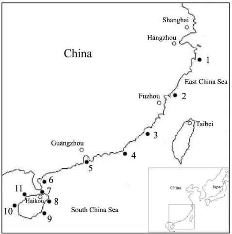
A total of 397 wild specimens of S. paramamosainwere collected from the following locations along the southeastern coast of China: Sanmen (SM, N38), Ningde (ND, N35), Zhangzhou (ZZ, N32), Shantou (ST, N25), Shenzhen (SZ, N40), Zhanjiang (ZJ, N41), Haikou (HK, N37), Wenchang (WC, N51), Wanning (WN,
N35), Dongfang (DF, N30) and Danzhou (DZ, N33) (Fig.1; Table1). Each specimen was killed by a lethal dose of MS-222. Genomic DNA was extracted from muscle tissue using traditional SUMMARY
The mud crab (Scylla paramamosain) is a carnivorous portunid crab, mainly distributed along the southeastern coast of China. Mitochondrial DNA analysis in a previous study indicated a high level of genetic diversity and a low level of genetic differentiation. In this study, population genetic diversity and differentiation of S. paramamosain were investigated using nine microsatellite markers. In total, 397 wild specimens from 11 locations on the southeastern coast of China were sampled and genotyped. A high level of genetic diversity was observed, with the number of alleles, and the observed and expected heterozygosity per location in the range 7.8–9.6, 0.62–0.77 and 0.66–0.76, respectively. AMOVA analysis indicated a low level of genetic differentiation among the 11 locations, despite the fact that a statistically significant fixation index (FST) value was found (FST0.0183, P<0.05). Out of 55 pairwise location comparisons, 39 showed significant FSTvalues (P<0.05), but all of them were lower than 0.05, except for one between Sanmen and Shantou locations. No significant deficiency of heterozygotes (inbreeding coefficientFIS0.0007, P>0.05) was detected for all locations except Sanmen and Zhanjiang. Cluster analysis using UPGMA showed that all locations fell into one group except Sanmen. Significant association was found between genetic differentiation in terms of FST/(1–FST) and the natural logarithm of geographical distance (r20.1139, P0.02), indicating that the genetic variation pattern closely resembled an isolation by distance model. This study supports the proposal of high genetic diversity and low genetic differentiation in S. paramamosain along the southeastern coast of China.
Key words: Scylla paramamosain, microsatellites, genetic diversity, genetic differentiation.
Received 23 February 2012: Accepted 11 May 2012 The Journal of Experimental Biology 215, 3120-3125
© 2012. Published by The Company of Biologists Ltd doi:10.1242/jeb.071654
RESEARCH ARTICLE
High genetic diversity and low differentiation in mud crab (Scylla paramamosain)
along the southeastern coast of China revealed by microsatellite markers
Hongyu Ma, Haiyu Cui, Chunyan Ma and Lingbo Ma*
Key Laboratory of East China Sea and Oceanic Fishery Resources Exploitation, Ministry of Agriculture, East China Sea Fisheries Research Institute, Chinese Academy of Fishery Sciences, Shanghai, 200090, China
proteinase K and phenol–chloroform extraction protocols as described previously (Ma et al., 2009). The DNA was adjusted to 100ngl–1and stored at –20°C until use.
Microsatellite genotyping
Nine polymorphic microsatellite loci were selected for genotyping, of which eight were developed using the 5⬘anchored PCR method (Cui et al., 2011), and the remaining one was developed using PCR-based isolation of microsatellite arrays (PIMA) (Ma et al., 2010) in our laboratory (Table2). The criteria for selection were as follows: annealing temperature of 50–63°C, expected product size between 110 and 320bp, observed heterozygosity value >0.5 and no stuttering bands. PCR reactions were conducted in a total volume of 25l and included 0.4moll–1each primer, 0.2mmoll–1each dNTP, 1⫻PCR
reaction buffer, 1.5mmoll–1 MgCl
2, 0.75U Taq polymerase and
approximately 100ng template DNA, under the following conditions: one cycle of denaturation at 94°C for 4min; 30 cycles
of 30s at 94°C, 50s at a primer-specific annealing temperature (Table2), and 50s at 72°C. As a final step, products were extended for 7min at 72°C.
Several methods, including agarose gel electrophoresis, denaturing polyacrylamide gel electrophoresis and automated DNA sequencing, were employed for detecting differences in nucleotide sequence, of which the second is a very effective and practical technique for genotyping of microsatellites and has been used in a wide range of organisms, as it has many advantages: a high resolution (about 1bp) and large output (100 samples each), low expense and easily mastered. In this study, the PCR products were separated on 6% denaturing polyacrylamide gels as described previously (Ma, 2009). The microsatellite fragments were visualized by silver staining, which was performed as follows. The gel was soaked in 1.0l staining solution (1.5g AgNO3) for about 10min;
this solution was then removed and the gel was washed in ddH2O
for 5s. Then the gel was soaked in 1.0l coloured solution (20g NaOH and 4ml formaldehyde) for about 10min. Finally, the gel was cleaned with ddH2O. The size of alleles was estimated according
to the pBR322/MspI marker.
Data analysis
Observed and expected heterozygosity, departure from Hardy–Weinberg equilibrium (HWE), linkage disequilibrium (LD) and inbreeding coefficient (FIS) were obtained using ARLEQUIN version 3.01 software (Excoffier et al., 2005). Genetic differentiation among locations was estimated using the analysis of molecular variance (AMOVA) approach by GENAlEX version 6.41 software (Peakall and Smouse, 2006). The significance levels were tested by 10,000 permutations for LD and by 1000 permutations for fixation index (FST) values. Observed number of alleles (Na), effective number of alleles (Ne) and genetic distance were estimated using POPGENE version 1.31 software (Yeh et al., 1999). An unweighted pair-group mean analysis (UPGMA) tree was constructed based on Nei’s genetic distance (Nei, 1978) of pairwise locations using MEGA version 4.0 software (Tamura et al., 2007). The association between genetic differentiation and geographic distance (isolation by distance) among locations was estimated by the Mantel test (Mantel, 1967) with 1000 permutations.
RESULTS
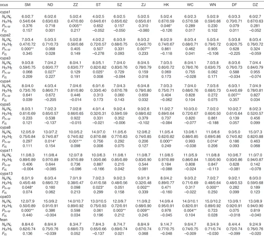
All nine microsatellite loci used in this study were polymorphic in each location, showing a high level of genetic diversity (Table3). In total, 104 alleles were detected from 397 individuals in 11 locations across nine loci. Naranged from six (Scypa1) to 16 (Scypa8 and Scpa03) per locus and from 7.8 (ST) to 9.6 (WC) per location.
HOand HE ranged from 0.32 to 1.00 and from 0.31 to 0.93 per locus–location combination, and from 0.62 (SM) to 0.77 (HK) and from 0.66 (ST) to 0.76 (ND and DZ) per location, respectively. FIS
ranged from –0.278 to 0.440 per locus–location combination and from –0.137 (ST) to 0.136 (SM) per location, with an average of 0.001 as a whole.
An exact probability test of HWE was performed among 99 locus–location combinations, and it revealed a significant deviation at 19 loci (P<0.05). These 19 loci were Scypa1 (in ZZ and HK), Scypa2 (in SM and ZJ), Scypa3 (in ND and ST), Scypa4 (in DF), Scypa8 (in ND, ZZ, HK and WN), Scypa13 (in SM, ST, ZJ and WN) and Scpa03 (in SM, SZ, ZJ and WC). Two loci (Scypa5 and Scypa11) were in keeping with HWE in all locations. Probability tests of genotypic LD for all pairs of loci within each location suggested significant non-random associations in only one of 396 possible pairwise comparisons after sequential Bonferroni correction
[image:2.612.52.291.68.310.2]Fig.1. Geographic map of southeastern coast of China. Filled circles, sampling location; 1, Sanmen (SM); 2, Ningde (ND); 3, Zhangzhou (ZZ); 4, Shantou (ST); 5, Shenzhen (SZ); 6, Zhanjiang (ZJ); 7, Haikou (HK); 8, Wenchang (WC); 9, Wanning (WN); 10, Dongfang (DF); and 11, Danzhou (DZ).
Table 1. Characteristics of 11 locations of Scylla paramamosain
Location Code Sample size Latitude (N) Longitude (E)
Sanmen SM 38 29°06⬙ 122°04⬙
Ningde ND 35 26°60⬙ 120°15⬙
Zhangzhou ZZ 32 24°27⬙ 118°17⬙
Shantou ST 25 23°16⬙ 116°84⬙
Shenzhen SZ 40 22°45⬙ 113°84⬙
Zhanjiang ZJ 41 21°04⬙ 110°58⬙
Haikou HK 37 20°12⬙ 110°34⬙
Wenchang WC 51 19°47⬙ 110°85⬙
Wanning WN 35 18°72⬙ 110°23⬙
Dongfang DF 30 19°26⬙ 108°30⬙
[image:2.612.45.295.623.745.2]Table 2. Characterization of the nine microsatellite markers used in this study
GenBank
Locus Repeat motifs Primer sequence (5⬘–3⬘) Ta(°C) accession no. References
Scypa1 (CTC)4TTC(CTC)2 CCCTACCTACCATTACACCC TATTACAAAGGACAGCCAGACA 54 HM623189 Cui et al., 2011
Scypa2 (GCA)13 TCTGTAATCAGACCAAGGAGGT CAAAATAGCCATACTGGAAGC 53 HM623190 Cui et al., 2011
Scypa3 (AGT)8 GCGGTTCATTTGCTTCG GAGACTGGGTTGTCCTTA 53 HM623191 Cui et al., 2011
Scypa4 (TCC)8N26(CTG)5 CTCCTGCCATCCTCATT AGCGGCATCTTTGTC 58 HM623192 Cui et al., 2011
Scypa5 (TAG)6TTG(TAG)2 ATAGTTGCTGGTTGATGAAG GGTCTGCGGCGAAT 54 HM623193 Cui et al., 2011
Scypa8 (CT)10 ACGAGACAGAGGGAGGC GGGTTCGAGATACAAGAT 63 HM623196 Cui et al., 2011
Scypa11 (CA)17N110(GTA)5 AACGCTACATCATACTGC CTGTTGCTATTTCTGCTT 50 HM623199 Cui et al., 2011
Scypa13 (AGG)8N10(AGG)4N3(AGG)3 CGTCTGTCCACCCTTAG CTTTCCCACAACCTCGTAT 61 HM623201 Cui et al., 2011
Scpa03 (TGTA)2N5(AT)4 CTGTAACACCCCAAAACAT GCCCAGGTACTCTCCACTC 52 GU182883 Ma et al., 2010
Ta, annealing temperature.
Table 3. Summary statistics of nine microsatellite markers in 11 locations of S. paramamosain
Locus SM ND ZZ ST SZ ZJ HK WC WN DF DZ
Scypa1
Na/Ne 6.0/2.7 6.0/2.6 5.0/2.4 4.0/2.5 6.0/2.5 5.0/2.5 5.0/2.4 6.0/2.3 5.0/2.9 6.0/3.3 6.0/2.7
HO/HE 0.54/0.64 0.63/0.63 0.47/0.60 0.64/0.61 0.65/0.62 0.65/0.61 0.67/0.59 0.57/0.58 0.59/0.66 0.70/0.71 0.67/0.63
PH–W 0.376 0.718 0.005** 0.652 0.157 0.310 0.046* 0.289 0.230 0.079 0.281
FIS 0.157 0.001 0.217 –0.052 –0.050 –0.060 –0.126 0.017 0.102 0.011 –0.052
Scypa2
Na/Ne 7.0/3.4 5.0/3.5 5.0/2.8 4.0/2.2 6.0/3.9 8.0/3.2 8.0/2.9 8.0/3.4 5.0/3.4 5.0/3.8 8.0/3.4
HO/HE 0.47/0.72 0.71/0.73 0.56/0.66 0.72/0.57 0.68/0.75 0.54/0.70 0.74/0.67 0.68/0.71 0.79/0.72 0.92/0.75 0.76/0.72
PH–W 0.000** 0.068 0.405 0.507 0.331 0.007** 0.861 0.462 0.905 0.628 0.324
FIS 0.345 0.028 0.149 –0.278 0.093 0.233 –0.118 0.041 –0.106 –0.225 –0.059
Scypa3
Na/Ne 9.0/3.8 7.0/4.2 8.0/4.1 8.0/5.1 7.0/4.0 8.0/4.5 7.0/3.5 8.0/4.1 7.0/3.8 8.0/3.6 7.0/4.4
HO/HE 0.59/0.75 0.60/0.77 0.63/0.77 0.82/0.82 0.83/0.76 0.78/0.79 0.60/0.72 0.78/0.76 0.63/0.75 0.76/0.73 0.84/0.79
PH–W 0.068 0.027* 0.129 0.025* 0.729 0.159 0.069 0.755 0.062 0.588 0.955
FIS 0.209 0.227 0.191 0.008 –0.094 0.018 0.173 –0.028 0.171 –0.034 –0.074
Scypa4
Na/Ne 8.0/4.0 4.0/3.4 7.0/4.6 6.0/1.6 7.0/4.3 6.0/4.8 7.0/3.3 7.0/4.0 7.0/3.6 6.0/3.1 7.0/4.9
HO/HE 0.73/0.76 0.86/0.71 0.81/0.80 0.33/0.40 0.67/0.78 0.78/0.80 0.75/0.71 0.68/0.76 0.68/0.73 0.44/0.69 0.78/0.81
PH–W 0.641 0.672 0.446 0.313 0.060 0.659 0.404 0.828 0.272 0.007** 0.827
FIS 0.039 –0.205 –0.014 0.173 0.143 0.032 –0.062 0.104 0.075 0.357 0.034
Scypa5
Na/Ne 8.0/3.1 7.0/2.3 7.0/2.8 4.0/1.4 9.0/2.4 9.0/2.6 11.0/2.7 10.0/3.0 7.0/2.0 10.0/2.7 8.0/2.3
HO/HE 0.61/0.69 0.65/0.57 0.66/0.65 0.32/0.31 0.59/0.59 0.68/0.62 0.69/0.64 0.72/0.67 0.60/0.50 0.61/0.64 0.52/0.57
PH–W 0.233 0.538 0.922 0.331 0.352 0.379 0.737 0.820 0.861 0.139 0.456
FIS 0.121 –0.137 –0.015 –0.021 –0.006 –0.102 –0.084 –0.077 –0.188 0.057 0.099
Scypa8
Na/Ne 12.0/5.9 13.0/7.2 10.0/5.2 14.0/7.0 11.0/5.6 12.0/6.2 11.0/5.4 13.0/6.1 11.0/6.6 9.0/5.0 15.0/7.3
HO/HE 0.75/0.84 0.74/0.87 0.74/0.82 0.87/0.88 0.77/0.83 0.74/0.85 0.62/0.82 0.88/0.85 0.69/0.86 0.74/0.82 0.82/0.88
PH–W 0.297 0.014* 0.001** 0.756 0.292 0.206 0.000** 0.993 0.014* 0.186 0.463
FIS 0.111 0.154 0.098 0.008 0.075 0.127 0.249 –0.038 0.206 0.093 0.068
Scypa11
Na/Ne 11.0/8.3 11.0/8.4 12.0/7.8 10.0/6.3 11.0/8.1 11.0/8.7 11.0/8.5 11.0/5.9 11.0/8.8 10.0/6.7 11.0/7.0
HO/HE 0.89/0.89 0.97/0.89 0.97/0.89 1.00/0.86 0.85/0.89 0.83/0.90 0.97/0.89 0.86/0.84 1.00/0.90 0.93/0.86 0.94/0.87
PH–W 0.406 0.644 0.736 0.887 0.215 0.544 0.184 0.808 0.847 0.628 0.142
FIS –0.004 –0.085 –0.096 –0.166 0.042 0.081 –0.088 –0.024 –0.113 –0.081 –0.078
Scypa13
Na/Ne 6.0/1.9 8.0/3.4 7.0/1.9 7.0/2.3 9.0/2.3 9.0/1.9 8.0/4.2 9.0/3.2 7.0/2.7 9.0/2.1 8.0/3.0
HO/HE 0.45/0.48 0.68/0.72 0.38/0.47 0.41/0.58 0.48/0.56 0.32/0.48 0.89/0.77 0.71/0.69 0.48/0.64 0.48/0.53 0.59/0.68
PH–W 0.048* 0.160 0.098 0.023* 0.051 0.002** 0.471 0.317 0.000** 0.282 0.189
FIS 0.074 0.062 0.213 0.299 0.158 0.339 –0.160 –0.022 0.250 0.099 0.123
Scpa03
Na/Ne 12.0/7.9 15.0/9.2 14.0/10.7 13.0/10.5 12.0/9.7 11.0/9.2 14.0/9.4 14.0/10.1 15.0/10.2 13.0/9.1 13.0/8.9
HO/HE 0.50/0.89 0.91/0.91 0.89/0.92 0.75/0.93 0.72/0.91 0.68/0.90 0.95/0.91 0.82/0.91 0.89/0.92 0.92/0.91 0.94/0.90
PH–W 0.000** 0.386 0.598 0.061 0.003** 0.009** 0.978 0.004** 0.723 0.075 0.819
FIS 0.440 –0.004 0.034 0.196 0.212 0.245 –0.045 0.104 0.028 –0.018 –0.040
Mean
Na/Ne 8.8/4.6 8.8/4.9 8.3/4.7 7.8/4.3 8.7/4.7 8.8/4.9 9.1/4.7 9.6/4.7 8.3/4.9 8.4/4.4 9.2/4.9
HO/HE 0.62/0.74 0.75/0.76 0.68/0.73 0.65/0.66 0.69/0.74 0.67/0.74 0.77/0.75 0.74/0.75 0.71/0.74 0.72/0.74 0.76/0.76
FIS 0.136 –0.039 0.052 –0.137 0.021 0.068 –0.048 –0.009 –0.030 –0.099 –0.020
For location names, see Table 1.
Na, observed number of alleles; Ne, effective number of alleles; HO, observed heterozygosity; HE, expected heterozygosity; PH–W, P-values for Hardy–Weinberg
equilibrium; FIS, inbreeding coefficient.
[image:3.612.51.565.240.702.2](Scypa2 and Scypa13 in DF, P<0.00139) (Rice, 1989). When each location was analysed separately, there was no evidence of stuttering and large allelic dropout in any of the loci, as confirmed by MICRO-CHECKER version 2.2.3 software (Van Oosterhout et al., 2004).
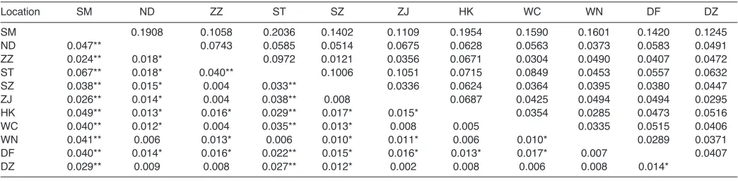
The AMOVA showed that genetic variation existed mainly within locations, rather than among locations, as the percentage of variance was 98.17% within locations and 1.83% among locations. Although the overall FST value for all locations and loci was statistically significant (FST0.0183, P<0.05), the genetic differentiation was still low, because the FSTvalue was much lower than 0.05 (Tables4, 5). Multi-locus estimates of FSTfor all possible pairwise locations ranged from 0.002 (ZJ and DZ) to 0.067 (SM and ST). The highest differentiation was between SM and ST (FST0.067), and the lowest differentiation was between ZJ and DZ (Table5). Thirty-nine out of 55 pairwise locations showed significant differentiation (P<0.05). Nei’s genetic distances between pairwise locations ranged from 0.0121 (ZZ and SZ) to 0.2036 (SM and ST), and were lower than 0.1 in 43 out of the 55 pairwise locations. Of the 11 locations, SM was the most distinctive, as it showed significant differentiation in relation to all the other 10 locations (FSTvalues ranged from 0.024 to 0.067). In contrast, DZ was the most representative as it significantly differed from only four locations (FSTvalues ranged from 0.012 to 0.029).
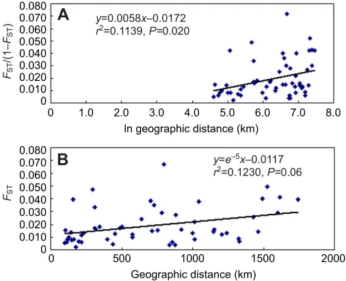
Cluster analysis of 11 locations using the UPGMA approach revealed two groups: one contained 10 locations and the other contained only one location (SM) (Fig.2). Mantel tests for isolation by distance among locations detected a significant positive correlation between pairwise FST/(1–FST) and the natural logarithm of geographic distance (km) (r20.1139, P0.02), while there was
no significant correlation between pairwise FST and geographic distance (km) (r20.1230, P0.06) (Fig.3)
DISCUSSION
The results of this study suggest a high level of population genetic diversity of S. paramamosainalong the southeastern coast of China (Na, HOand HEin the range 7.8–9.6, 0.62–0.77 and 0.66–0.76 per location, respectively), in accordance with previous studies that showed a high level of mtDNA genetic diversity in S. paramamosain
(Lu et al., 2009; Ma et al., 2011a). High population genetic diversity has also been observed in other marine animals, such as scallop (Chlamys farreri) (Zhao et al., 2009), Atlantic salmon (Salmo salar) (Karlsson et al., 2010) and silver pomfret (Pampus argenteus) (Zhao et al., 2011). Three factors including the life history characteristics, environmental heterogeneity and large population size may help to maintain a high level of genetic diversity (Perrine, 1979; Nei, 1987; Avise, 1998). On the whole, the level of genetic diversity of S. paramamosainfrom the southern regions was higher than that from the northern regions (Table3), which may be due to the different environments. A similar finding was observed in a previous study, which indicated a trend for a reduction in genetic diversity of S. paramamosainfrom south to north, step by step using mtDNA (Lu et al., 2009).
Generally, marine fishes are considered to have a low level of genetic differentiation among different geographic populations because of the high dispersal capabilities, large population sizes and relatively small barriers in the marine environment (Beheregaray and Sunnucks, 2001). For the fish Nibea albiflora, there was little
SZ ZZ WC ZJ DZ DF WN HK ND ST SM
0 0.02
0.04 0.06
0.080 0.070 0.060 0.050 0.040 0.030 0.020 0.010 0
0 1.0 2.0 3.0 4.0
ln geographic distance (km)
5.0 6.0 7.0 8.0
0 500 1000 1500
Geographic distance (km)
2000 0.080
0.070 0.060 0.050 0.040 0.030 0.020 0.010 0
A
B
y=0.0058x–0.0172
r2=0.1139, P=0.020
y=e–5x–0.0117 r2=0.1230, P=0.06 FST
/(1–
FST
)
FST
Fig.2. The unweighted pair-group mean analysis (UPGMA) tree of 11 locations of Scylla paramamosain. SM, Sanmen; ND, Ningde; ZZ, Zhangzhou; ST, Shantou; SZ, Shenzhen; ZJ, Zhanjiang; HK, Haikou; WC, Wenchang; WN, Wanning; DF, Dongfang; and DZ, Danzhou.
Fig.3. Relationship between genetic differentiation and geographic distance among the 11 locations. (A)Relationship between pairwise FST/(1–FST)
(where FSTis the fixation index) and the natural logarithm of geographic
[image:4.612.48.279.67.218.2]distance. (B)Relationship between pairwise FSTand geographic distance.
Table 4. AMOVA design and results for 11 locations of S. paramamosain
Source of variation d.f. Sum of squares Variance components % variation FST
Among locations 10 83.706 0.064 1.83 0.0183
Among individuals within locations 386 1465.290 0.388 11.18
Within individuals 397 1199.000 3.020 86.99
Total 793 2747.996 3.472 100
[image:4.612.314.567.71.276.2] [image:4.612.47.569.673.731.2]difference in the population genetic structure between the Yellow Sea and East China Sea observed using mtDNA (Han et al., 2008). For the shrimp Fenneropenaeus chinensis, no significant population genetic differentiation between the Yellow Sea and Bohai Sea was found using both microsatellite DNA and mtDNA (Liu et al., 2006; Li et al., 2009b). For the crab S. paramamosain, a genetically homogeneous population structure with high gene flow was observed among most localities along the coasts of the East China Sea and South China Sea using mtDNA (He et al., 2010). In the current study, statistically significant genetic differentiation was detected across 11 locations along the southeastern coast of China (FST0.0183, P<0.05), but the FST value was still low (<0.05), suggesting a low level of genetic differentiation (Wright, 1978). A similar finding was reported in earlier studies, which suggested a low differentiation in S. paramamosainusing mtDNA (Lu et al., 2009; He et al., 2010; Ma et al., 2011a). The above information indicates that all locations of S. paramamosainshould be a single genetically homogeneous population. The low FSTvalue indicates a relatively high gene flow among locations. There are three probable explanations for this: (1) the unique reproductive habit in which adults and juveniles migrate between ocean basins and adjacent continental margins; (2) the high dispersal capabilities of larvae; and (3) the relatively small physical barriers in the marine environment.
Among these 11 locations, SM was the most genetically distinctive in two main ways: (1) it has the lowest genetic diversity (the overall HOwas 0.62) and the highest FSTvalues (between 0.024 and 0.067) compared with other locations; and (2) it has the greatest overall FISvalue (FIS0.136, P<0.05) compared with other locations. These findings indicate that the gene exchange is relatively low between SM and other locations compared with that between other location pairs. The optimum temperature range of this crab is 18–27°C for growth, and a higher temperature is needed for spawning. However, SM is the most northern of these locations, so the seawater temperature is the lowest in the same period. Low temperature may limit the effective population size and the high dispersal capabilities of S. paramamosain. Over-fishing by humans may be another potential explanation. A significant positive correlation between genetic differentiation and geographic distance was found, suggesting an isolation by distance model of genetic variation.
CONCLUSIONS
In conclusion, a high level of population genetic diversity and low differentiation were found in the mud crab (S. paramamosain) from 11 locations along the southeastern coastal regions of China by
microsatellite analysis, which showed a genetically homogeneous population structure for S. paramamosainin these 11 locations. In the future, more population genetic studies should be carried out in this crab species. The findings in this study will provide valuable information for conservation, harvesting and artificial selective breeding of this important fishery resource.
LIST OF ABBREVIATIONS
AMOVA analysis of molecular variance
FIS inbreeding coefficient
FST fixation index
HE expected heterozygosity
HO observed heterozygosity
HWE Hardy–Weinberg equilibrium
LD linkage disequilibrium
Na observed number of alleles
Ne expected number of alleles
ACKNOWLEDGEMENTS
We thank Dr Keji Jiang for assistance in partial sample collection.
FUNDING
This research was supported by the National Non-Profit Institutes (East China Sea Fisheries Research Institute) [grant no. 2011M05], the National Natural Science Foundation of China [grant no. 31001106], and the Science and Technology Commission of Shanghai Municipality [grant no. 10JC1418600].
REFERENCES
Avise, J.(1998). Phylogeography. Cambridge, MA: Harvard University Press.
Beheregaray, L. B. and Sunnucks, P.(2001). Fine-scale genetic structure, estuarine colonization and incipient speciation in the marine silverside fish Odontesthes
argentinensis. Mol. Ecol.10, 2849-2866.
Cui, H. Y., Ma, H. Y., Ma, L. B., Ma, C. Y. and Ma, Q. Q.(2011). Development of eighteen polymorphic microsatellite markers in Scylla paramamosainby 5⬘anchored PCR technique. Mol. Biol. Rep.38, 4999-5002.
Dickerson, B. R., Ream, R. R., Vignieri, S. N. and Bentzen, P.(2010). Population structure as revealed by mtDNA and microsatellites in northern fur seals, Callorhinus
ursinus, throughout their range. PLoS ONE5, e10671.
Dudaniec, R. Y., Storfer, A., Spear, S. F. and Richardson, J. S.(2010). New microsatellite markers for examining genetic variation in peripheral and core populations of the coastal giant salamander (Dicamptodon tenebrosus). PLoS ONE 5, e14333.
Excoffier, L., Laval, G. and Schneider, S.(2005). ARLEQUIN (version 3.0): an integrated software package for population genetics data analysis. Evol. Bioinform.
Online1, 47-50.
Gvozdík, V., Moravec, J., Klütsch, C. and Kotlík, P.(2010). Phylogeography of the Middle Eastern tree frogs (Hyla, Hylidae, Amphibia) as inferred from nuclear and mitochondrial DNA variation, with a description of a new species. Mol. Phylogenet.
Evol.55, 1146-1166.
Han, Z. Q., Gao, T. X., Yanagimoto, T. and Sakurai, Y.(2008). Genetic population structure of Nibea albiflorain the Yellow Sea and East China Sea. Fish. Sci.74, 544-552.
He, L., Zhang, A., Weese, D., Zhu, C., Jiang, C. and Qiao, Z.(2010). Late Pleistocene population expansion of Scylla paramamosainalong the coast of China: a population dynamic response to the last interglacial sea level highstand. J. Exp.
[image:5.612.45.567.79.207.2]Mar. Biol. Ecol.385, 20-28.
Table 5. Pairwise FST(below diagonal) and genetic distance (above diagonal) among the 11 locations of S. paramamosain
Location SM ND ZZ ST SZ ZJ HK WC WN DF DZ
SM 0.1908 0.1058 0.2036 0.1402 0.1109 0.1954 0.1590 0.1601 0.1420 0.1245 ND 0.047** 0.0743 0.0585 0.0514 0.0675 0.0628 0.0563 0.0373 0.0583 0.0491 ZZ 0.024** 0.018* 0.0972 0.0121 0.0356 0.0671 0.0304 0.0490 0.0407 0.0472 ST 0.067** 0.018* 0.040** 0.1006 0.1051 0.0715 0.0849 0.0453 0.0557 0.0632 SZ 0.038** 0.015* 0.004 0.033** 0.0336 0.0624 0.0364 0.0395 0.0380 0.0447 ZJ 0.026** 0.014* 0.004 0.038** 0.008 0.0687 0.0425 0.0494 0.0494 0.0295 HK 0.049** 0.013* 0.016* 0.029** 0.017* 0.015* 0.0354 0.0285 0.0473 0.0516 WC 0.040** 0.012* 0.004 0.035** 0.013* 0.008 0.005 0.0335 0.0515 0.0406 WN 0.041** 0.006 0.013* 0.006 0.010* 0.011* 0.006 0.010* 0.0289 0.0371 DF 0.040** 0.014* 0.016* 0.022** 0.015* 0.016* 0.013* 0.017* 0.007 0.0407 DZ 0.029** 0.009 0.008 0.027** 0.012* 0.002 0.008 0.006 0.008 0.014*
Karlsson, S., Moen, T. and Hindar, K.(2010). Contrasting patterns of gene diversity between microsatellites and mitochondrial SNPs in farm and wild Atlantic salmon.
Conserv. Genet.11, 571-582.
Keenan, C. and Blackshaw, P. A.(1999). Mud Crab Aquaculture and Biology. ACAIR Proceedings No. 78. Australia: Watson Ferguson & Co.
Li, M. H., Välimäki, K., Piha, M., Pakkala, T. and Merilä, J.(2009a). Extrapair paternity and maternity in the three-toed woodpecker, Picoides tridactylus: insights from microsatellite-based parentage analysis. PLoS ONE4, e7895.
Li, Y. L., Kong, X. Y., Yu, Z. N., Kong, J., Ma, S. and Chen, L. M.(2009b). Genetic diversity and historical demography of Chinese shrimp Fenneropenaeus chinensisin Yellow Sea and Bohai Sea based on mitochondrial DNA analysis. Afr. J. Biotechnol. 8, 1193-1202.
Liu, P., Meng, X. H., Kong, J., He, Y. Y. and Wang, Q. Y. (2006). Polymorphic analysis of microsatellite DNA in wild populations of Chinese shrimp
(Fenneropenaeus chinensis). Aqua. Res.37, 556-562.
Lu, X. P., Ma, L. B., Qiao, Z. G., Zhang, F. Y. and Ma, C. Y.(2009). Population genetic structure of Scylla paramamosainfrom the coast of the Southeastern China based on mtDNA COI sequences. J. Fish. China.33, 15-23. (In Chinese with English abstract.)
Ma, H. Y.(2009). Development of sex-specific markers and ssr markers and construction of genetic linkage maps of three important cultured marine fish species. PhD thesis, Ocean University of China, Qingdao, China.
Ma, H. Y., Yang, J. F., Su, P. Z. and Chen, S. L.(2009). Genetic analysis of gynogenetic and common populations of Verasper moseriusing SSR markers.
Wuhan Univ. J. Nat. Sci.14, 267-273.
Ma, H. Y., Ma, C. Y., Ma, L. B. and Cui, H. Y.(2010). Novel polymorphic microsatellite makers in Scylla paramamosainand cross-species amplification in related crab species. J. Crustac. Biol.30, 441-444.
Ma, H. Y., Ma, C. Y. and Ma, L. B.(2011a). Population genetic diversity of mud crab
(Scylla paramamosain) in Hainan Island of China based on mitochondrial DNA.
Biochem. Syst. Ecol.39, 434-440.
Ma, H. Y., Chen, S. L., Yang, J. F., Chen, S. Q. and Liu, H. W.(2011b). Genetic linkage maps of barfin flounder (Verasper moseri) and spotted halibut (Verasper
variegatus) based on AFLP and microsatellite markers. Mol. Biol. Rep.38,
4749-4764.
Ma, H. Y., Ma, C. Y. and Ma, L. B.(2011c). Identification of type I microsatellite markers associated with genes and ESTs in Scylla paramamosain. Biochem. Syst.
Ecol.39, 371-376.
Mantel, N.(1967). The detection of disease clustering and a generalized regression approach. Cancer Res.27, 209-220.
Nei, M.(1978). Estimation of average heterozygosity and genetic distance from a small number of individuals. Genetics89, 583-590.
Nei, M.(1987). Molecular Evolutionary Genetics. New York, NY: Columbia University Press.
Ortega-Villaizan Romo, M., Suzuki, S., Nakajima, M. and Taniguchi, N.(2006). Genetic evaluation of interindividual relatedness for broodstock management of the rare species barfin flounder Verasper moseriusing microsatellite DNA markers. Fish. Sci.72, 33-39.
Peakall, R. and Smouse, P. E.(2006). GENALEX 6: genetic analysis in excel. Population genetic software for teaching and research. Mol. Ecol. Notes6, 288-295.
Perrine, D.(1979). The Mangrove Crab on Ponape.88 pp. Ponape Eastern Caroline Islands: Marine Resources Division.
Rice, W. R.(1989). Analyzing tables of statistical tests. Evolution43, 223-225.
Shen, Y. and Lai, Q.(1994). Present status of mangrove crab (Scylla serrata
(Forskål)) culture in China. NAGA: the ICLARM Quarterly, January 1994, 28-29.
Takano, M., Barinova, A., Sugaya, T., Obata, Y., Watanabe, T., Ikeda, M. and Taniguchi, N.(2005). Isolation and characterization of microsatellite DNA markers from mangrove crab, Scylla paramamosain. Mol. Ecol. Notes5, 794-795.
Tamura, K., Dudley, J., Nei, M. and Kumar, S.(2007). MEGA4: molecular
evolutionary genetics anlysis (MEGA) software version 4.0. Mol. Biol. Evol.24, 1596-1599.
Van Oosterhout, C., Hutchinson, W. F., Wills, D. P. M. and Shipley, P.(2004). MICRO-CHECKER: software for identifying and correcting genotyping errors in mirosatellite data. Mol. Ecol. Notes4, 535-538.
Van Syoc, R. J., Fernandes, J. N., Carrison, D. A. and Grosberg, R. K.(2010). Molecular phylogenetics and biogeography of Pollicipes(Crustacea: Cirripedia), a Tethyan relict. J. Exp. Mar. Biol. Ecol.392, 193-199.
Wright, S.(1978). Evolution and the Genetics of Populations, Vol. 4, Variability Within
and Among Natural Populations. Chicago: The University of Chicago Press.
Yeh, F. C., Yang, R. C. and Boyle, T.(1999). POPGENE version 1.31. Microsoft
window-based freeware for population genetic analysis. University of Alberta and the
Centre for International Forestry Research. Available at www.ualberta.ca/~fyeh/.
Zhang, Y., Xu, P., Lu, C., Kuang, Y., Zhang, X., Cao, D., Li, C., Chang, Y., Hou, N., Li, H. et al.(2011). Genetic linkage mapping and analysis of muscle fiber-related QTLs in common carp (Cyprinus carpioL.). Mar. Biotechnol. (NY)13, 376-392.
Zhao, C., Li, Q. and Kong, L.(2009). Inheritance of AFLP markers and their use for genetic diversity analysis in wild and farmed scallop (Chlamys farreri). Aquaculture 287, 67-74.