University of Pennsylvania
ScholarlyCommons
Publicly Accessible Penn Dissertations
1-1-2016
Essays on the Estimation of Demand for
Complementary Goods
Ludovic Stourm
University of Pennsylvania, [email protected]
Follow this and additional works at:
http://repository.upenn.edu/edissertations
Part of the
Advertising and Promotion Management Commons
, and the
Marketing Commons
Recommended Citation
Stourm, Ludovic, "Essays on the Estimation of Demand for Complementary Goods" (2016).Publicly Accessible Penn Dissertations. 2042.
Essays on the Estimation of Demand for Complementary Goods
Abstract
This dissertation investigates the problem of demand estimation across complementary goods at the level of individual purchase decisions made by consumers. At this micro level, package sizes may restrict the amount of goods that can be purchased, and temporary price discounts may induce consumers to stockpile goods in anticipation of their future consumption needs, leading to dynamics in purchasing behavior over time. We address these issues in two essays by proposing new structural models of demand. In the first essay, we develop a new approach to modeling consumer preferences for complements which is based on household production theory, and we study the importance of accounting for package size restrictions in modeling cross-category price effects. In the second essay, we embed this approach in a model of consumer forward-looking behavior to study the consequences of stockpiling behavior on the spillover effect of prices across
complementary products that are storable.
Degree Type Dissertation
Degree Name
Doctor of Philosophy (PhD)
Graduate Group Marketing
First Advisor Raghuram Iyengar
Second Advisor Eric T. Bradlow
Subject Categories
ESSAYS ON THE ESTIMATION OF DEMAND FOR COMPLEMENTARY GOODS
Ludovic Stourm
A DISSERTATION
in
Marketing
For the Graduate Group in Managerial Science and Applied Economics
Presented to the Faculties of the University of Pennsylvania
in
Partial Fulfillment of the Requirements for the
Degree of Doctor of Philosophy
2016
Supervisor of Dissertation
Raghuram Iyengar,
Associate Professor of Marketing
Co-Supervisor of Dissertation
Eric T. Bradlow,
K. P. Chao Professor of Marketing, Statistics and Education
Graduate Group Chairperson
Eric T. Bradlow, K. P. Chao Professor of Marketing, Statistics and Education
Dissertation Committee
David R. Bell, Xinmei Zhang and Yongge Dai Professor of Marketing
ESSAYS ON THE ESTIMATION OF DEMAND FOR COMPLEMENTARY GOODS
c
COPYRIGHT
2016
Ludovic Stourm
This work is licensed under the
Creative Commons Attribution
NonCommercial-ShareAlike 3.0
License
ACKNOWLEDGEMENT
During the four years I spent in Wharton’s Ph.D. program, I met some very talented people
that I wish to acknowledge for their help and support. I could have not completed the PhD
program without them, and it is not without nostalgia that I am preparing to leave Wharton
to start a new adventure.
First and foremost, I would like to thank my co-advisors Raghu Iyengar and Eric Bradlow
for their support, endless energy and availability. In our weekly meetings, we have had
insightful discussions and I have learned a lot about research.
I also want to extend warm thanks to my other committee members David Bell and
Jean-Fran¸cois Houde. David gave me thorough advice on my dissertation idea early in the
program, and the directions he suggested have guided me in the development of my
disser-tation. Jean-Fran¸cois gave me crucial advice on methodological issues and his expertise in
industrial organization has been invaluable.
Other faculty members gave me insightful feedback at various stages of my dissertation,
whose names deserve to be acknowledged: Josh Eliashberg, Dave Reibstein, Pete Fader and
Bob Meyer. More generally, the current dissertation benefited from comments that were
brought up by the faculty and students during my presentations in Wharton’s Marketing
Department and I am very grateful for these.
This work would have not been possible without the funding I received from the Jay H.
Baker Retailing Center, for which I am very grateful. I am also indebted to the James M.
Kilts Center for Marketing at Chicago Booth for giving me access to the data I used in my
dissertation. I also want to thank my former boss Steve Cohen and the team at In4mation
Insights, who first introduced me to marketing research and supported my decision to pursue
past) that I have met during my time at Wharton, who have contributed to make each day
more enjoyable in the office.
Last but not least, I want to thank my wife Valeria for her support. I could have not
ABSTRACT
ESSAYS ON THE ESTIMATION OF DEMAND FOR COMPLEMENTARY GOODS
Ludovic Stourm
Raghuram Iyengar
Eric T. Bradlow
This dissertation investigates the problem of demand estimation across complementary
goods at the level of individual purchase decisions made by consumers. At this micro level,
package sizes may restrict the amount of goods that can be purchased, and temporary
price discounts may induce consumers to stockpile goods in anticipation of their future
consumption needs, leading to dynamics in purchasing behavior over time. We address these
issues in two essays by proposing new structural models of demand. In the first essay, we
develop a new approach to modeling consumer preferences for complements which is based
on household production theory, and we study the importance of accounting for package
size restrictions in modeling cross-category price effects. In the second essay, we embed this
approach in a model of consumer forward-looking behavior to study the consequences of
stockpiling behavior on the spillover effect of prices across complementary products that
TABLE OF CONTENTS
ACKNOWLEDGEMENT . . . iii
ABSTRACT . . . v
LIST OF TABLES . . . viii
LIST OF ILLUSTRATIONS . . . ix
CHAPTER 1 : The importance and challenges of modeling demand for complements 1 CHAPTER 2 : A Flexible Demand Model for Complements Using Household Pro-duction Theory . . . 4
2.1 Motivation . . . 4
2.2 Formalization and literature . . . 7
2.3 Model . . . 10
2.4 Econometric model . . . 19
2.5 Simulation study . . . 23
2.6 Empirical application . . . 27
2.7 Conclusion . . . 34
CHAPTER 3 : A Dynamic Model of Purchase and Consumption Across Comple-mentary Categories . . . 36
3.1 Motivation . . . 36
3.2 Literature . . . 38
3.3 Model . . . 42
3.4 Simulation study . . . 52
3.5 Empirical application . . . 57
CHAPTER 4 : General Conclusion . . . 67
APPENDIX . . . 71
LIST OF TABLES
TABLE 1 : Results of a simulation study under the household-production model
of complementarity . . . 25
TABLE 2 : Description of purchase data in the tortilla chips and Mexican salsa
categories . . . 29
TABLE 3 : Reduced-form evidence of complementarity between tortilla chips
and Mexican salsa . . . 29
TABLE 4 : Estimation results on the tortilla chips and Mexican salsa purchase
data . . . 30
TABLE 5 : Results of counterfactual analyses under alternative couponing
strate-gies . . . 33
TABLE 6 : Integrating the literature on cross-category demand estimation and
the literature on stockpiling behavior . . . 39
TABLE 7 : Simulation results under different versions of the dynamic
cross-category model of demand . . . 54
TABLE 8 : Description of purchase data in the spaghetti and tomato sauce
cat-egories . . . 59
TABLE 9 : Reduced-form analysis of stockpiling behavior . . . 59
TABLE 10 : Reduced-form analysis of complementarity between spaghetti and
tomato sauce . . . 61
TABLE 11 : Estimates of the price process parameters . . . 62
LIST OF ILLUSTRATIONS
FIGURE 1 : Relationship between ˜U, U and V in the household-production
model of complementarity . . . 12
FIGURE 2 : Indifference curves under various parameter values . . . 16
FIGURE 3 : Consumption policy under various parameter values . . . 49
FIGURE 4 : Effect of an exogenous promotion on sales across categories in
sim-ulated data . . . 57
FIGURE 5 : Effect of exogenous promotions on sales of spaghetti and tomato
CHAPTER 1 : The importance and challenges of modeling demand for complements
This chapter motivates the importance of modeling demand for complementary goods in
marketing, reviews the related literature, introduces some of the challenges in doing so, and
gives an overview of how we tackle them in the next two chapters.
Understanding how demand responds to marketing activity is crucial for any successful
marketing action. In today’s world, companies record data about individual purchases
made by their customers, and can leverage this historical data to get insight about their
preferences and purchasing behavior. Companies can then use this knowledge to make
better decisions about their marketing mix, for example by optimizing their prices or their
promotion schedules to achieve a higher profit. For retailers and manufacturers who produce
multiple goods, it is important to understand how their marketing mix affects demand
across related categories, since their total profit depend on their joint sales. Therefore,
they can better coordinate their marketing strategy by analyzing purchase data across
categories. The first part in implementing such a data-driven strategy consists in estimating
an empirical model of demand on the data. It is particularly important to have a good model
of demand because it is used as input for the evaluation of any alternative marketing plan:
as such, the optimal marketing action derives directly from it.
Micro-level models of demand, where each individual consumer purchase decision is
mod-eled, present at least two important advantages over macro-level models of demand, where
demand is aggregated over consumers and/or time periods in some pre-defined markets.
First, it is important for marketers to understand consumer heterogeneity, so that the
mar-keting mix can be tailored to the specific needs of individual consumers. For example,
companies target their customers when sending promotional coupons, or propose different
versions of their products to capture different segments of consumers. Macro-level models
of demand cannot give insights about such consumer heterogeneity, since they only
and relates to the estimation of the model: as explained by Lucas (1976), aggregate-level
empirical models yield parameter estimates that are not invariant to policy changes. In
a marketing context, this means that the parameters of the model depend on the current
marketing mix: if some aspects of the marketing mix are changed, then the parameter
es-timates are no longer accurate. This can be problematic since the purpose of the analysis
is usually to evaluate alternative marketing strategies. On the other hand, it is possible to
specify a micro-level model of consumer behavior based on economic theory such that its
parameters are invariant to policy changes.
In the marketing literature, the first demand model applied on micro-level scanner data was
the logit model by Guadagni and Little (1983) to investigate consumer choices of brands
within a product category. Many models have been developed since then to capture
con-sumer heterogeneity (Kamakura and Russell, 1989; Rossi et al., 1996), to model concon-sumers’
purchase incidence and quantity decisions (Chintagunta, 1993), and to capture dynamic
behavior over time such as learning (Erdem and Keane, 1996) or stockpiling (Erdem et al.,
2003; Sun, 2005). A stream of research has also emerged to model cross-category demand,
with the goal of measuring the spillover effect of marketing activity and prices across
re-lated product categories (Mehta, 2007; Song and Chintagunta, 2007). Unlike brands within
a product category, which are typically substitutes, different categories may be substitutable
or complementary: under the usual definition from economics, they may exhibit positive or
negative cross price effects on demand.
As noted by Berry et al. (2014), many empirical tools to study demand for substitutable
goods have been developed, but the estimation of demand for complements still presents
some methodological challenges. While the starting point of a micro-level demand system
derived from first economic principles is that the consumer maximizes her utility or stream
of utilities defined on goods purchased, the problem of specifying a parametric form for
models have relied on additional assumptions to derive a demand system, such as
continu-ous quantities or sequential decision processes (Mehta, 2007; Song and Chintagunta, 2007;
Mehta and Ma, 2012; Lee and Allenby, 2014).
This dissertation proposes a new approach to modeling demand for complements by
invok-ing household production theory. Under that view, consumers purchase goods to use them
as inputs to produce final goods, and they derive utility by consuming these final goods.
In Chapter 2, we show that representing consumer preferences for latent final goods
con-sumed instead of the goods purchased can yield a flexible utility function that can capture
complementarity, using very simple parametric forms. We then study the properties of the
resulting demand system in a static model with independent purchase occasions, and
esti-mate the model on data to show how it can be used for coordinated pricing and packaging
decisions across complementary categories. In Chapter 3, we embed our utility
specifica-tion in a dynamic model of cross-category purchase and consumpspecifica-tion where consumers are
forward-looking and can store goods between time periods. Through simulation and in a
real data application, we investigate the importance of accounting for consumer stockpiling
CHAPTER 2 : A Flexible Demand Model for Complements Using Household
Production Theory
2.1. Motivation
Consumers commonly purchase multiple goods to consume them jointly. For example,
they buy burgers and buns to make sandwiches, they combine detergent and softener for
their laundry, or eat crackers with dips. From a managerial point of view, cross-category
consumption provides an opportunity for coordinated promotion and pricing across the
goods. A rigorous analysis of optimal marketing strategy first requires a model of demand
in a way that takes into account the volumes purchased by consumers across categories.
Not surprisingly, modeling demand across categories has therefore been an important area
of research in the marketing literature.
By leveraging household-level data of purchases made across categories and over time,
mar-keting researchers have built models to estimate demand at the micro level (Manchanda
et al., 1999; Song and Chintagunta, 2007; Mehta, 2007; Niraj et al., 2008; Mehta and Ma,
2012; Lee et al., 2013). Many of these econometric models take a utility-maximization
paradigm to obtain parameters that are invariant to policy changes. In this paradigm, the
starting point is that consumers choose to buy the quantities of goods that maximize their
utility under a budget constraint. The goal of estimation is therefore to find the
param-eters of the model that best explain the purchases observed, under the assumption that
these purchases are the result of an optimization problem. From this common setup, two
approaches have been developed, which differ in what economic object is parameterized.
Both approaches have advantages and limitations.
In the first approach, the researcher specifies a functional form for the indirect utility and
applies Roy’s identity (Roy, 1947) to derive the demand function, which relates the
complementarity and/or substitution across goods, Roy’s identity only applies if any
con-tinuous quantity can be demanded, and if prices are linear in quantity. These assumptions
may lead to biases when demand is indivisible due to package size constraints (Lee and
Allenby, 2014).
In the second approach, the researcher parameterizes the consumer’s direct utility function
and solves the first-order conditions to obtain the demand function. The model can then
be easily extended to include richer aspects of the world, such as discrete package sizes.
However, it is difficult to find a functional form for the direct utility that is tractable (in the
sense that the first-order conditions can be solved easily), regular (in the sense that it yields
well-behaved preferences on the entire domain of preference parameters), and flexible (in
the sense that it can accommodate different patterns of consumer preferences and demand
functions). This is problematic: a non-flexible functional form may lead to a poor model
of demand if it is unable to capture a pattern that exists in the data. Additively-separable
specifications, which are the most tractable, cannot lead to complementarity between goods,
as defined by negative cross price effects (Chintagunta and Nair, 2011). For that reason,
cross-category demand models often take the indirect utility approach.
In this chapter, we propose a new model of demand for complementary goods in a way that
yields flexible patterns, yet can be used in contexts where Roy’s identity does not apply.
Our approach relies on household production theory (Muth, 1966): the original consumer
problem is altered to distinguish between inputs that can be purchased and latent final
goods that can be consumed. We represent the joint consumption of multiple inputs by
a separate final good: for example, buns and burgers can be purchased (and consumed
separately), but sandwiches need to be produced from buns and burgers. Formally, the
consumer has a utility function defined on goods consumed (e.g. sandwiches, burgers and
buns), but can only buy inputs (e.g. burgers and buns). She decides not only what inputs
to purchase but also what final goods to produce for her own consumption. This conceptual
goods purchased, but it is more general if we assume that a broader set of final goods can
be produced from the goods purchased.
Even though consumption may not be observable, we find that it is useful to lay out the
consumer problem in this way to obtain a parametric representation of consumer
prefer-ences for observables that yields a flexible demand system. We show that a direct utility
defined oninputs can always be derived from our model, although its functional form is not
straightforward. In contrast, even a separately-additive functional form for the utility on
final goods can capture very different patterns of preferences, including perfect
complemen-tarity, asymmetric complementarity or no complementarity. Thus, representing consumer
preferences for latent final goods instead of inputs greatly facilitates the problem of finding
a flexible, tractable and regular functional form.
We consider three different versions of our model: one version where the consumer can
purchase any continuous quantities of goods, one version where demand is restricted to lie
on a discrete grid of points due to package size constraints, and one version where demand
is discrete but we shut off complementarity by removing any joint consumption as a final
good. We derive some insights about the properties of our demand system by studying
the continuous model since the corresponding consumer problem can be solved analytically.
In a simulation study, we investigate the consequences of ignoring (or allowing for)
dis-creteness and complementarity between goods in the estimation of own- and cross-category
price effects, and we show that our model recognizes the absence of complementarity when
demand is independent across goods. In an empirical application, we estimate our models
on purchase data from a panel of consumers over time, focusing on the tortilla chips and
Mexican salsa categories. We find that ignoring the discreteness of demand leads to very
different inferences about cross-price elasticities, which is of particularly interesting since
most previous multicategory models of demand take the indirect-utility approach and
consumers.
The rest of the chapter is organized as follows. In Section 2.2, we formalize the economic
problem of a consumer making quantity choices across related goods, and review the
econo-metric models that have been derived from it in the marketing literature. In Section 2.3, we
lay out a more general model of consumer behavior based on household production theory,
and show its usefulness for empirical work by studying its properties. In Section 2.4, we
in-troduce stochasticity in the model, and discuss its identification and estimation. Section 2.5
describes the results of a simulation study that compares our model against extant research.
In Section 2.6, we describe an application of our model on household-level purchase data,
and show how it can inform managerial decisions. Section 2.7 concludes with a discussion
of the main contributions and limitations of our model, and ideas for future research.
2.2. Formalization and literature
Suppose we want to model the purchase decisions of a consumer acrossJ goods of interest.
In the simplest microeconomic model, the consumer has a utility function U defined on
the quantities of these goods x= (x1, ..., xJ) and the quantityz of an outside good. After
observing the prices p, she chooses to buy the quantities that maximize her utility within
her budget M. Mathematically, the consumer problem is represented as:
V(p, M) = max
x∈X,z≥0 U(x, z)
subject to: p(x) +z≤M
(2.1)
wherex belongs to some set X,p(x) is the dollar amount to be paid to buy the quantities
x of inside goods, and where the price of the outside good is normalized to one. In this
maximization problem, U is the direct utility, V is the indirect utility, and the demand
function x∗(p, M) gives the optimal quantities. From the observation of prices and the
quantities purchased by consumers, the goal of demand estimation consists in characterizing
demand under alternative scenarios with different pricesp, budgetM, or constraints on the
set X.
Empirically estimating a demand model requires one to make parametric assumptions which
should lead to a tractable, flexible and regular demand system. Finding such a functional
form turns out to be challenging in the case of complementary goods. Previous marketing
literature has addressed it in two different ways, by either specifying a functional form for
the indirect utilityV or for the direct utilityU. The article by Chintagunta and Nair (2011)
provides an excellent review of that literature.
In the indirect-utility approach, the researcher specifies a functional form for V, typically
using the translog function which can approximate any twice continuously differentiable
functionV at a second degree (Song and Chintagunta, 2007; Mehta, 2007; Mehta and Ma,
2012). Under the assumptions that prices are linear in quantity (p(x) =P
jxjpj), and that
any non-negative quantities can be demanded (X =RJ+), the researcher then applies Roy’s
identity to obtain the demand function: x∗j = −∂V /∂pj
∂V /∂M. The estimation problem consists
in finding those parameters of V that best fit the data. This approach has been used to
model demand across substitutable and complementary categories, providing an integrated
framework for purchase incidence, volume and brand decisions (Song and Chintagunta,
2007; Mehta, 2007; Mehta and Ma, 2012). Parameterizing the indirect utility V bypasses
the problem of specifying a functional form for the direct utility U and is thought to be a
more flexible approach since the indirect utility can always be derived from a direct utility
specification but the reverse is not true. However, the underlying properties of consumer
preferences are not clear and may lead to regularity problems: the demand function may
not always exhibit some desirable properties, such as homogeneity of degree zero. In a
recent article, Mehta (2015) alleviates some of these concerns by studying the conditions on
the specification that are necessary and sufficient for regularity. Nevertheless, this approach
In a second approach pioneered by Kim et al. (2002), the researcher specifies a functional
form for the direct utility U and derives the demand function by solving the first-order
conditions of the consumer problem in Equation 2.1. This approach is appealing because
it allows one to accommodate different pricing schemes and/or constraints present in the
real world by changing the feasible set X and the price function p. For example, Satomura
et al. (2011) allow for multiple constraints (such as a volume constraint) instead of a
sin-gle budget constraint; Lee et al. (2014) capture the indivisibility of demand by including
integer constraints on the feasible set. Through these extensions, researchers have gained
a richer understanding of the impact of prices and packaging on demand. However, one
major hurdle consists in finding a parameterization of U that yields flexible patterns of
demand. Chintagunta and Nair (2011) show that, under linear prices, additively
separa-ble utility functions of the form Ux(x1, ..., xJ) = PJj=1φj(xj) can only yield nonnegative
cross effects of prices on demand, thus ruling out complementarity between the goods. On
the other hand, non-additively separable utility functions may be intractable or may not
exhibit desired properties of regularity for all parameter values, such as monotonicity and
concavity. Thus finding a parametric form ofU to capture complementarity is difficult. Lee
et al. (2013) circumvent this problem by assuming a sequential decision process whereby
consumers make purchase decisions one category at a time: at each stage, the consumer
maximizes a category-specific utility function that may be affected by purchase decisions in
previous categories through an effect of inventories. Such sequential decisions are
charac-teristic of lexicographic preferences, which cannot be represented by a joint utility function
defined on the entire set of goods.
We develop a third approach, which relies on the household production theory introduced
by Muth (1966). In this view, households buy inputs to produce final goods that they
consume: as such, they are both producers (with a production function that transforms
inputs into final goods) and consumers (with a utility function defined on final goods). In
our context, we argue that complementary goods can be consumed either separately, or
purchased, and each consumption use (separate or joint) as a different final good. Thus two
goods can be complementary if the consumer uses them jointly to construct a final good
from which she enjoys utility.
Even though consumer preferences are only revealed through purchase behavior in the
absence of consumption data, we show that it is useful to represent consumer preferences
over consumption bundles to obtain a flexible system of demand for goods purchased, which
is amenable for estimation in the presence of indivisibility constraints and corner solutions.
Our work is closely related to the latent separability concept defined by Blundell and Robin
(2000), which is a property of direct utility functions. Like the authors, we recognize that
parts of the same input can be allocated to different final goods. For example, consumers
may eat some burgers by themselves, and combine some with buns to make sandwiches.
Unlike Blundell and Robin (2000) however, we do not require fewer final goods than inputs:
in fact, we include more final goods than inputs. This is because they seek to reduce the
dimensionality of the demand system by grouping goods into latent groups while we aim
at flexibly estimating the demand across a narrower set of goods. Section 2.3 describes our
model in more depth.
2.3. Model
We start by laying out the general model of household production and explain how it
relates to the direct-utility approach and the indirect utility approach. Then we describe
our parametric assumptions, study the implications of the resulting model for consumer
preferences over goods purchased, and its implications for the demand function under the
assumptions of Roy’s identity.
2.3.1. Consumer problem with household production
By considering household production, we make a conceptual distinction between theinputs
and buns which are sold separately on the market, but in order to eat a sandwich, she first
needs to produce it by combining a bun and a burger. In this example, burgers and buns
are inputs, and sandwiches are final goods. We denote byJ the number of distinct inputs,
by K the number of distinct final goods that can be produced from the J inputs, by
x = (x1, ..., xJ) the volumes of inputs purchased and by c = (c1, ..., cK) the quantities of
final goods consumed. Importantly, the consumer first needs to buy enough inputs to be
able to produce the final goods. To do so, she has a budget M that she can spend across
the inputs and to buy some quantityzof an outside good whose price is normalized to one.
The consumer enjoys utility from consuming the final goods and the outside good, which
is represented by a utility function ˜U(c, z). The consumer problem consists in buying the
optimal volumes of inputsx and outside goodz, and use the inputs to produce the optimal
quantities of final goodsc in a way that maximizes her utility1:
V(p, M) = max
c,x,z
˜
U(c, z)
subject to: p(x) +z≤M
x∈ X
c∈ C(x)
(2.2)
wherep(x) is the dollar amount to be paid by the consumer if she buys the volumes of inputs
x, and C(x) is the set of final goods that can possibly be produced from them. Clearly, the
consumer makes the best use of her inputs by allocating them into the production of the
optimal quantities of final goods. Thus, the value that the consumer can derive from input
quantities xand outside good quantity z can be obtained as:
U(x, z) = max
c
˜
U(c, z)
subject to: c∈ C(x)
(2.3)
Under this definition of U(x, z), the consumer problem in Equation 2.2 can be rewritten
under the form of Equation 2.1. From the point of view of the consumer’s purchase behavior,
our model is thus equivalent to the original problem considered in Equation 2.1. However,
adding a production-consumption step allows us to parameterize ˜U(c, z) andC(x) instead
of U(x, z) in the direct-utility approach, orV(p, M) in the indirect-utility approach. The
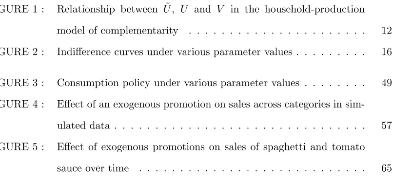
relationship between ˜U(c, z),U(x, z) andV(p, M) is explained in Figure 1. In our approach,
we specify a functional form on ˜U(c, z) and solve the problem in Equation 2.2 to derive the
demand function x∗(p, M). It should be noted that, if we assume C(x) to be the identity
correspondence (C(x) ={x} ∀x, so that there is no difference between goods purchased and
goods consumed), then Equation 2.3 trivially implies U(x, z) = ˜U(c, z). It is thus obvious
that any parameterization ofU(x, z) in a direct-utility model can easily be accommodated
under our approach by settingC(x) to be the identity correspondence. In contrast, Equation
2.3 implies that a utility function over goods purchasedU(x, z) can always be inferred from
a utility function over goods consumed ˜U(c, z); however, the derived expression of U may
not be straightforward. Since preferences are only revealed through the purchase of inputs
in the absence of consumption data, only properties ofx∗(p, M) can be identified from the
data. Yet, parameterizing ˜U(c, z) andC(x) instead ofU(x, z) can be much more convenient
as we show in the next sections, because it allows us to derive a flexible and regular demand
function using very simple parametric forms.
!"($, &)
!((, &)
)(*, +)
,(()
X, +, *(()
(
∗(*, +)
Optimal
consumption
problem
Optimal
purchase
problem
2.3.2. Parametric assumptions
We represent the joint consumption of multiple goods as a separate final good, which is
obtained by combining inputs in fixed proportions. We also allow each good to be consumed
separately. Thus, the same input can be used to produce different final goods, and some
final goods may require multiple inputs. We represent this by a Leontief production function
that can be described by aJ xKinput-output table, denoted byA, such thatajkrepresents
the volume of inputj that is required to make one unit of final goodk. For example, the
input-output table may look like the following in the case of burgers and buns:
A=
sandwich burg. only bun only
burger 1 1 0
bun 1 0 1
(2.4)
The set C(x) of final good quantities c that can be produced from input volumes x is the
set of vectorscwith nonnegative entries and such thatP
kajkck≤xj for allj, or in matrix
form: Ac≤x.
Next, we parameterize the utility function for goods consumed as follows:
˜
U(c, z) = ˜Uc(c) +Uz(z) (2.5a)
with : U˜c(c) =
K
X
k=1
αklog(ck+ 1) (2.5b)
Uz(z) =α0z (2.5c)
where α1, ..., αK and α0 are parameters whose values are nonnegative. This form is
com-monly used to parameterize the utility for goods purchasedU(x, z) in direct-utility models
of demand (Satomura et al., 2011; Lee et al., 2013; Lee and Allenby, 2014). It has
de-sirable properties: the log function captures monotonicity and concavity in its argument,
this functional form is additively separable, which makes it easy to solve the consumer
problem but implies that a model where this form is used to parameterize U(x, z) cannot
capture complementarity between theJ goods of interest. Since we use it to parameterize
˜
U(c, z) instead, the resulting model can actually capture very flexible models of demand for
complements, as we show in the next two sections.2
2.3.3. Implications for consumer preferences over goods purchased
In this section, we show how our model of preferences over final goods translates into
preferences over goods purchased. Using Equation 2.3 and Equations 2.5a-2.5c, our
param-eterization of ˜U(c, z), implies the following utility for purchased goodsU(x, z):
U(x, z) =Ux(x) +Uz(z) (2.6a)
where Ux(x) = max c
K
X
k=1
αklog(ck+ 1) (2.6b)
subject to: X
k
ajkck≤xj ∀j (2.6c)
ck ≥0 ∀k (2.6d)
Equations 2.6b-2.6d define the consumer’s problem of optimally allocating inputs to
con-struct final goods. This problem is mathematically very similar to the multiple-constraint
model by Satomura et al. (2012), except that there is no outside good added for each linear
constraint in Equation 2.6c. The first-order conditions of the optimal allocation problem
2
In previous literature, the utility for the outside good is sometimes specified asUz(z) =α0log(z), to
are as follows:
αk
ck+ 1
+λk−
X
j
µjajk = 0 ∀k
λkck = 0 ∀k
µj xj−
X
k
ajkck
!
= 0 ∀j
ck, µk, λj ≥0
(2.7)
where the coefficientsλkandµjare Lagrange multipliers corresponding to the non-negativity
constraints on the quantities of final goodsck and the constraints on the amount of inputs
available, respectively. In a case with J = 2 inputs and K = 3 final goods such that
A=
1 0 1
0 1 a23
, we can easily obtain the expression of the optimal quantities of final
goods consumed as a function of the quantities of goods purchased:
c∗3(x) = min
max
0, c(int)3 (x)
, x1,
x2
a23
c∗1(x) =x1−c∗3
c∗2(x) =x2−a23c∗3
(2.8)
where c(int)3 is the solution to a second-degree equation, as shown in Appendix A.1. The
resulting utility over inputs purchased is thenUx(x) =Uc(c∗(x)).3
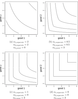
Using the expression of Ux, we illustrate in Figure 2 several patterns of indifference curves
obtained from our model with different parameter values, holding the outside good constant
and focusing on Ux. As we can see, our model is very flexible: it can accommodate very
different patterns of preferences from perfect complementarity to no complementarity, with
symmetry or asymmetry.
3One may argue that we could have directly parameterized the utility for inputs purchasedU
x(x) using
that expression, without laying out the household production problem. While it is true that the resulting
demand system would be the same, we emphasize that the derived expression ofUx(x) is not straightforward
and cannot be simplified, while our parameterization ofUc(c) has a closed-form expression. Thus setting up
Figure 2: Indifference curves under various parameter values
good 1
good 2
2
4
6
0 1 2 3 4
0
1
2
3
4
(a)α1,separate= 2
α2,separate= 2
α3,joint= 0
good 1
good 2
1 2 3
4
0 1 2 3 4
0
1
2
3
4
(b)α1,separate= 0.5
α2,separate= 0.5
α3,joint= 3
good 1
good 2
1 2 3
4
0 1 2 3 4
0
1
2
3
4
(c)α1,separate= 1
α2,separate= 0
α3,joint= 3
good 1
good 2
1 2 3 4
0 1 2 3 4
0
1
2
3
4
(d)α1,separate= 0
α2,separate= 0
α3,joint= 3
2.3.4. Implications for demand under continuous quantities
In this section, we study the properties of the demand functionx∗(p, M) under the
assump-tion of linear prices (such that p(x) = P
jpjxj), and assuming that the J inputs can be
purchased in any nonnegative, continuous quantities (such that X =RJ+). In this case, the
demand function can be solved easily and we can obtain intuitive insights into its
proper-ties. Since any continuous quantities of inputs can be purchased, the consumer will buy
the quantities that are exactly necessary to make the optimal quantities c∗k of final goods:
buying more inputs would only come at a monetary cost. Thus the demand for inputs must
be such that:
x∗j =
K
X
k=1
akjc∗k ∀j (2.9)
Furthermore, we can define the full price fk of each final good k as the dollar amount
that the consumer needs to pay to produce one unit of that final good, by buying all the
necessary inputs:
fk= J
X
j=1
akjpj (2.10)
By using this definition, the consumer problem in Equation 2.2 can be simplified and
rewrit-ten in terms of the final goods only:
max
c,z
˜
U(c, z)
s.t.
K
X
k=1
fkck+z≤M
(2.11)
The first-order conditions can then be solved to obtain the optimal quantities of final goods
under our parameterization of ˜U(c, z):
c∗k = max
0,αk fk
−1
The demand function is obtained by combining Equations 2.9 and 2.3.4. We can then use
these results to study the effect of input prices on demand for theJ inputs:
∂x∗j ∂pj0 =
∂PK
k=1akjc∗k
∂pj0
=X
k
akj
∂c∗k ∂pj0
=X
k
akj
∂c∗k ∂fk
× ∂fk ∂pj0
=X
k
akjakj0
∂c∗k ∂fk
=−X
k
akjakj0αk
fk2I(pk< αk)
(2.13)
where I(.) is the indicator function. If j = j0, then clearly the derivative is negative,
which implies that own price effects are negative. IfA is the identity matrix (which means
that C(x) is the identity correspondence, and there is no final good representing a joint
consumption), then the cross price effects are zero, since ajj0 = 0 if j 6=j0. However, if it
is not the case, then we should expect negative cross price effects when two goods j and
j0 are jointly used as inputs to produce at least one final good k, such that akj > 0 and
akj0 > 0. Thus, by specifying a consumer problem in the space of final goods and then
aggregating demand across these final goods to obtain the demand for inputs, we capture
complementarity between the goods purchased.
Let us consider again the case withJ = 2 inside goods andK = 3 final goods, where the first
two final goods correspond to the separate consumption of each inside good and the third
one is a composite final good that corresponds to their joint consumption. Let us assume
that the composite final good is obtained by combining the inputs in the same proportions,
such thata23= 1. When the utility parameter for the composite final good is positive and
good, and the consumer simply considers the “full price” of the composite final good and
decides what quantityc3 to produce and consume of it. In that case, a one-dollar increase
in the price of one input leads to a one-dollar increase in the full price of the composite final
good, which may lead the consumer to reduce the quantityc∗3 of composite final good and
therefore the quantities of both inputs purchased by the same amount. Mathematically,
Equation 2.13 implies that ∂x
∗
1
∂p1 =
∂x∗1
∂p2 =
∂x∗2 ∂p1 =
∂x∗2
∂p2 =−
α3
f2
3 in that case. Thus a one-dollar price change of each input should have the same effect on demand across all inputs: the
own- and cross- price effects should be the same and should all be equal across theJ goods.
Alternatively, if the consumer has positive utilities for some of the inputs consumed
sep-arately (α1 > p1 and/or α2 > p2), then the own- price effects and the cross- price effects
may be different because some of the inputs may be consumed by themselves. In that case,
the price of good 1 impacts the demand for good 2 only to the extent that it impacts their
joint consumption (whose utility is captured byα3). On the other hand, the price of good 2
impacts the demand for good 2 both because it impacts the consumption of good 2 by itself
(whose utility is captured by α2) and the joint consumption with good 1. If the separate
consumption of the inputs give different utilities (such thatα16=α2), then the cross- price
effects may be asymmetric. Thus, our model of household production provides an intuitive
explanation for the existence of asymmetric cross- price effects between goods.
2.4. Econometric model
In this section, we describe how we apply our model to data. We first introduce stochastic
elements to allow for consumer heterogeneity and variation of preferences over time. Then
we focus on the estimation of the model of demand under the assumption of continuous
demand. Next, we relax the assumption of infinitely divisible demand. Finally, we discuss
2.4.1. Distributional assumptions
We now introduce the subscript i to refer to a consumer, and the subscript t to indicate
a specific purchase occasion. Suppose that we follow N consumers, each over Ti purchase
occasions: we observe the pricespitthat they face, and the volumes of goods xijt that they
purchase. We take a random-utility approach to rationalize these purchase decisions under
the consumer problem in Equation 2.2, by including random shocks in the consumer’s utility
function. Specifically, we assume that the α parameters of consumer i at time t are such
that:
αikt =αikeikt
where ikt iid
∼N(0, σ2)
(2.14)
The values αik represents the stable part of the consumer’s preferences and the shocks
ikt capture variation over time. The model only makes sense if the preference parameters
αik are non-negative: thus we consider their log. We collect all individual-level preference
parameters into a vectorωi, and model unobserved consumer heterogeneity through random
coefficients:
ωi iid∼M V N(¯ω, V)
whereωi = [log(αi1), ...,log(αiK)]
(2.15)
The resulting model is a hierarchical Bayesian model where consumer i’s contribution to
the likelihood can be written as follows:
Li(ωi, σ2) = Ti
Y
t=1
Z
it
" Y
k
φ
1
σikt
#
I
x∗(ωi, it|pit) =xit dit (2.16)
where I(.) is the indicator function, it is a collection of all the shocks ikt, x∗(ωi, it|pit)
is the optimal demand under price function pit and shocks it, and φ is the pdf of the
standard Normal distribution. The difficult part in evaluating the likelihood consists in
2.4.2. Model with continuous quantities
In this section, we discuss the estimation of the model considered in Section 2.3.4, where
each goodjhas a unit price equal topjand can be purchased in any nonnegative, continuous
quantity. As explained earlier, we can define a full price fk for one unit of each final good
k using Equation 2.11. Let us suppose for a moment that we can observe the quantities of
final goodsciktproduced by consumeriat timet. Then, from Equations 2.3.4 and 2.14, we
can derive either an upper bound or an exact value for the random utility shocks:
ikt ≤log fikt αik
ifcikt= 0
= log
fikt
αik
×(cikt+ 1)
ifcikt>0
(2.17)
We can use this result to compute the probability that the quantities of final goodscikt are
optimal under preference parametersωi and prices pit:
P r(c) =
Y
ks.t. ck=0
Φ 1 σ log fikt αik Y
ks.t.ck>0
1 σφ 1 σlog fikt αik
×(ck+ 1)
1
ck+ 1
(2.18)
where Φ is the cdf of the standard Normal distribution, and the term c1
k+1 on the right
side is a Jacobian due to the transformation from the random shocksto the quantities of
final goodsc. Since consumption is unobserved, we need to integrate this probability over
the possible set of final good quantities, conditional on the observed quantities purchased
xj. From Equation 2.9, we must havexj =Pkajkck, or in matrix notation: x=Ac where
ck ≥0 for all k. Thus, we have an aggregate data problem: we have a complete likelihood
defined over the consumption of final goods ck (Equation 2.18), but we only observe the
volumes of inputs purchased xj, which are an aggregation of those final goods. We can
rewrite consumeri’s contribution to the likelihood as:
Li(ωi, σ2) = Ti
Y
t=1
Z
c≥0 s.t.Ac=xit
P r c∗(ωi, pit) =c
In the case of two inputs and three final goods, we only need to integrate out c3 since c1
andc2 can be obtained directly fromc3 and x. Still, this integration is not straightforward.
To estimate the model, we apply data augmentation (Tanner and Wong, 1987), treatingc3
as the augmented data.
2.4.3. Model with indivisible demand
We now relax the assumptions of continuous purchases, and consider a situation in which
each good is sold as a package containing a volume sj, with a unit price equal to pj. The
consumer can then choose to buy any integer number qj of packs for goodj. Under these
assumptions, we have:
qj ∈ {0,1,2, ...}∀j (2.20a)
xj =qjsj (2.20b)
p(x) =X
j
qjpj (2.20c)
This new setup allows us to accommodate the indivisibility of demand, as the possible
quantities purchased by the consumer lie on a grid of discrete points defined by the integer
constraints on the quantities of packs qj. The consumer problem 2.2 can no longer be
simplified to obtain a closed-form expression for the demand x∗, like it was the case under
continuous quantities. We must then evaluate the consumer’s objective function on all
such points (assuming a reasonable upper bound on the number of packsqj), and find that
point which yields the highest value to obtain the demand x∗. Furthermore, the integral
in Equation 2.16 cannot be simplified, thus we apply data augmentation to estimate the
model, by treatingzikt = log(αik) +iktas the augmented data. Our approach is similar to
2.4.4. Identification
We discuss how the parameters of our model can be identified from patterns of purchases as
a function of prices, in the absence of consumption data. We assume that the consumer’s
budget M is large enough so that it does not restrict the amount of inputs purchased but
only the amount of outside good; consequently, it drops out of the consumer problem.4
Theαkparameters capture the consumer’s utility for final goods: as such, they are defined
relative to the marginal utility for the outside good α0, and we fix their scale by setting
α0 = 1. Different values of αk yield different own- and cross- price effects, as discussed in
Section 2.3.4. Thus they are identified by the own- and cross- effects of prices on purchases;
the magnitude of the price effects are smaller when theαk parameters are larger. Separate
from cross- price effects, correlation in purchases is captured through the random shocks.
In the analyses that follow, we consider a case with J = 2 inputs and K = 3 final goods,
with the assumption that A =
1 0 1
0 1 1
.
5 The variation in purchase behavior at the
individual level can be disentangled from consumer heterogeneity since we have panel data
with a time series of observations for each consumer.
2.5. Simulation study
We ran a simulation study to investigate how the assumption of continuous demand may
affect the parameter estimates of our model and the inferences drawn regarding the effect of
prices on demand. We also sought to investigate the possible consequences of ignoring (or
allowing for) complementarity between goods when estimating demand. For this analysis,
we considered three different versions of our proposed model. Model 1 is a restricted version
of our discrete model where we shut off any complementarity between goods by removing
the possibility of joint consumption: in this model, the final goods are equivalent to the
4
This is an assumption commonly made in the literature (see Lee et al., 2013, for example).
5The proportions used in combining both inputs for a joint consumption, captured bya
23, can be treated
as a parameter to estimate. In theory, it can be identified through the proportions in which goods are purchased but in practice, it may be difficult to identify it when there is not much variation in quantities purchased, which is the case in our empirical application. Future research should consider the consequences
inputs purchased, thus K=J and Ais the identity matrix. Model 2 is our discrete model
that allows for complementarity, as laid out in Section 2.4.3. Model 3 is the continuous
version of our model, as laid out in Section 2.4.2. For each model, we used the hierarchical
Bayesian paradigm to model consumer heterogeneity.
We generated a dataset for each of the three models, using that model as the true data
generating process. We defined a set of J = 2 goods purchased, each good being sold
in a pack of size one under Model 1 and Model 2, or in any continuous quantities under
Model 3. We generated the preference parameters of 200 consumers from a multivariate
normal distribution with mean ¯ω and covariance matrix V, where ¯ω and V were drawn in
a way that yields a reasonable amount of variation in purchase behavior.6 Unit prices were
drawn from a uniform distribution in interval [0.2,1.2]. For each consumer, we generated
100 purchase occasions, and solved for the optimal purchase quantities using either a grid
search (for Models 1 and 2) or the first-order conditions (for Model 3). Each resulting
dataset contained the prices observed by consumers and the quantities purchased of each
good. For each consumer, we used the first 100 purchase occasions for model estimation,
We estimated the three models on the datasets generated under Model 1 and Model 2.
While demand is discrete in these datasets, Model 3 disregards package size constraints
and assumes that the quantities purchased are exactly the continuous quantities desired
by consumers. Reversely, Models 1 and 2 cannot accommodate the continuous quantities
present in the dataset generated under Model 3, therefore we only applied Model 3 on
that dataset, with the objective of verifying that we can recover the true parameters. The
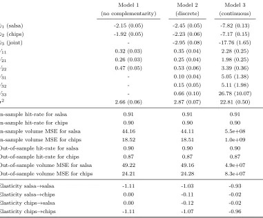
estimation results are compiled in Table 1. The first set of rows indicates our estimates of the
average preference parameters ¯ω along with their posterior standard error in parentheses.
The second set of rows gives in-sample and out-of-sample model fit criteria: for each good,
the hit-rate of predicted purchase incidence and mean squared error of volume purchased
averaged across all purchase occasions and consumers. The last set of rows gives an estimate
of own- and cross- price elasticities, obtained by simulating the aggregate demand under a
10% price increase for each good.
We can make several observations from these results. First, we recovered the true parameters
within their 95% posterior intervals for each dataset when estimating the “true” model,
and the “true” model made predictions that were better or at least as good as the other
models, both in-sample and out-of-sample. While expected, these results confirm that the
parameters of our model can be empirically identified and that our estimation procedure
can recover them.
The estimation results also provide insights about the effect of capturing or ignoring
comple-mentarity between the goods. The first dataset was generated according to Model 1, which
does not have any complementarity between goods purchased. However, it should be noted
that Model 3, which allows for such complementarity, accurately estimates the true
pref-erence parameters for separate consumptions ¯ω1 and ¯ω2 and yields a very low estimate for
the preference parameter of the joint consumption ¯ω3. With such a low preference for joint
joint consumption does not exist. Thus the model yields accurate own- price elasticities,
and cross- price elasticities equal to zero. Reversely, the second dataset was generated
un-der the assumption of a joint consumption having a relatively high utility compared to the
separate consumption of the goods, as indicated by the high value of ¯ω3. This leads to
the existence of negative cross- price effects, as shown by the sign of the true cross- price
elasticities. On that dataset, the model that does not allow for complementarity (Model 1)
leads to a bias in the estimation of of own- price elasticities. Taken together, these results
suggest that if there is no complementarity, the model that allows for complementarity
yields correct estimates of own- and cross- price effects, but if there exist complementarity,
then a model that ignores it not only yields cross- price elasticities equal to zero, but also
a biased estimate of own- price elasticities.
We can also get some insights about the importance of accounting for the indivisibility
of demand by looking at the estimation results of the continuous model (Model 3) on
the second dataset, which is generated according to the discrete model (Model 2). The
only difference between the two models is that Model 3 does not take into account the
discreteness implied by package size constraints. As we can see, ignoring indivisibility
leads to an underestimation of all preference parameters. This result is consistent with the
article by Lee and Allenby (2014): in a model of continuous demand, consumers should buy
a positive quantity of each good (even very small) unless the good gives a smaller marginal
utility than her marginal utility of money: consequently, such a model rationalizes a low
purchase incidence rate by a very small marginal utility for the good when in fact, the low
purchase incidence rate may due to large packages. In our simulation, the own- and
cross-price elasticities we found were still similar under the continuous and the discrete model,
which may be explained by the relatively small package size we assumed.
2.6. Empirical application
This section discusses an application of our model on a real dataset from a panel of
this analysis, we sought to evaluate the fit of our model against a set of competing models,
and to show how the results can be used to help make better managerial decisions. We first
describe the data, then we present our estimation results, and finally we illustrate the
use-fulness of our model through counterfactual analyses studying the effect of different types
of coupons.
2.6.1. Data
The data was collected by AC Nielsen and is made of two parts. The first part contains
data about a set of households who report their purchases over time using a scanner device
at home: it provides the information about all shopping trips made by the households,
the number of units purchased and the price paid for each item purchased. Prices are
only observable when a purchase is made, therefore we combine the data about households
with the second part of the data, which gives us store-level prices for each item each week.
We chose the tortilla chips and Mexican salsa categories for our empirical application, and
focused on a two-year time window from 2010 to 2011. We focused respectively on the
10-ounce and 16-10-ounce package sizes, which are the predominant formats in these categories.
We aggregated prices at the category level by taking an average of brand-specific prices
weighed by market share. We restricted the data to households making at least 8 purchases
in each of the two categories over the two-year period.
The resulting dataset contained 251 consumers, each consumer making 151 shopping trips
on average. Table 2 gives some summary statistics of the data. Consumers bought multiple
units of chips or salsa in 30% of their purchases, which indicates the need for a model of
quantity. Consumers often bought both goods together, as indicated by the high percentage
of purchase co-incidence relative to the marginal percentages of incidence. We ran logit
models of incidence for each category to investigate the effect of prices on demand, with
(a) Purchase frequency
Salsa and chips Salsa only Chips only None
Number of observations (%) 1187 (3.1%) 2218 (5.9%) 2878 (7.6%) 31625 (83.4%)
(b) Descriptive statistics
Salsa Chips
Price ($) 2.70 2.60
Purchase incidence (%) 8.98 10.72
Mean purchase quantity 1.34 1.32
Table 2: Description of purchase data in the tortilla chips and Mexican salsa categories
Incidence of salsa Incidence of salsa (with household FE)
Salsa price -0.4381 (0.0905) -0.6294 (0.1206)
Chips price -0.2934 (0.0552) -0.2797 (0.0782)
Incidence of chips Incidence of chips (with household FE)
Salsa price -0.2572 (0.0847) 0.0192 (0.1171)
Chips price -0.7411 (0.0524) -0.9065 (0.0749)
Table 3: Reduced-form evidence of complementarity between tortilla chips and Mexican salsa
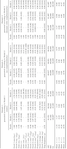
2.6.2. Estimation results
We estimated several models on the data: the discrete model that rules out complementarity
(Model 1), our discrete model of complementary demand based on household production
theory (Model 2) and the continuous version of that model (Model 3). For each model, we
used a Bayesian estimation procedure to generate 500,000 draws of the parameters from
their posterior distribution. We discarded the first 100,000 draws and kept one draw every
100 draws thereafter to reduce autocorrelation. We ran three separate chains to assess
convergence.
Comparing model fits is difficult because the Deviance Information Criterion (DIC), which
is usually used in model selection between hierarchical Bayesian models, requires one to
evaluate the likelihood at the average posterior draw of all parameters. Since we also
draw the random shocks as augmented data, we would need to evaluate the likelihood at
the average of the random shocks, individual- and population-level preference parameters
Model 1 Model 2 Model 3
(no complementarity) (discrete) (continuous)
¯
ω1 (salsa) -2.15 (0.05) -2.45 (0.05) -7.82 (0.13)
¯
ω2 (chips) -1.92 (0.05) -2.23 (0.06) -7.17 (0.15)
¯
ω3 (joint) - -2.95 (0.08) -17.76 (1.65)
V11 0.32 (0.03) 0.35 (0.04) 2.28 (0.25)
V21 0.26 (0.03) 0.25 (0.04) 1.98 (0.25)
V22 0.47 (0.05) 0.53 (0.06) 3.39 (0.36)
V31 - 0.10 (0.04) 5.05 (1.38)
V32 - 0.15 (0.05) 5.11 (1.98)
V33 - 0.66 (0.10) 26.78 (10.07)
σ2 2.66 (0.06) 2.87 (0.07) 22.81 (0.50)
In-sample hit-rate for salsa 0.91 0.91 0.91
In-sample hit-rate for chips 0.90 0.90 0.90
In-sample volume MSE for salsa 44.16 44.11 5.5e+08
In-sample volume MSE for chips 18.52 18.51 1.0e+09
Out-of-sample hit-rate for salsa 0.90 0.90 0.90
Out-of-sample hit-rate for chips 0.87 0.87 0.87
Out-of-sample volume MSE for salsa 49.22 49.16 4.9e+07
Out-of-sample volume MSE for chips 24.21 24.28 8.3e+07
Elasticity salsa→salsa -1.11 -1.03 -0.93
Elasticity salsa→chips 0.00 -0.11 -0.02
Elasticity chips→salsa 0.00 -0.12 -0.02
Elasticity chips→chips -1.11 -1.07 -0.96
the observed actions are optimal, which implies that the likelihood of an observed action is
equal to one conditional on posterior random shocks and posterior preference parameters.
However, this property may no longer be true when averaging across draws, leading to a
likelihood equal to 0 at the “average draw” and thus a DIC equal to minus infinity.
Instead of likelihood-based criteria, we relied on in-sample and out-of-sample predictions to
compare model fits. Specifically, we predicted purchase incidence and volumes purchased
(in ounces) for each consumer trip, for each of the two goods. To make predictions, we
drew random shocks from their prior distribution and determined the optimal purchase
action conditional on our posterior draws of the consumer’s preference parameters and the
prior random shocks drawn. We predicted a purchase incidence when the probability of a
purchase was at least 50%. The hit-rate was obtained as the percentage of correct incidence
predictions. It should be noted that the actual incidence rates are quite low in the data,
and therefore it is easy to obtain a high hit-rate by simply predicting no incidence at every
shopping trip. For that reason, we also report the mean squared error (MSE) of our volume
predictions.
In Table 4, we have compiled for each model, our estimates of the population-level mean
parameters along with the corresponding posterior standard deviation in parentheses. We
have also reported the results of our predictions, as well as own- and cross-price elasticities.
Price elasticities were computed by simulating a 10% increase in the price of each good and
determining the aggregate demand under each alternative scenario, based on the posterior
draws of the random shocks and of the individual-level preference parameters.
The continuous model’s predictions are clearly worse than those obtained from the other
two models, as the high estimated variance for the random shocks leads to very large
pre-dictions. Compared to the discrete model, the average preference parameters ¯ωk are again
under-estimated in the continuous model. The continuous model also yields much smaller
cross- price elasticities, which is particularly interesting since most multicategory models in
bias may lead to suboptimal marketing decisions from retailers and manufacturers.
Our model and the no-complementarity model yield similar fits in terms of predictions
both in-sample and out-of-sample. However, the no-complementarity model cannot explain
the reduced-form evidence of cross- price effects shown in Section 2.6.1. Furthermore,
the estimates of preference parameters ¯ω1 and ¯ω2 are significantly different across the two
models, unlike what we obtained in the simulation study described in Section 2.5, where
our discrete model recovered the true values of ¯ω1 and ¯ω2 and yielded a very low value for
¯
ω3 when data was generated according to the no-complementarity model. This suggests
that our discrete model captures complementarity that is present in the data. The
own-price elasticities obtained are somewhat similar across the two models but our discrete
model yields non-negligible cross-price elasticities, which could lead to different price and
promotion decisions across the two categories.
2.6.3. Counterfactuals
We now illustrate how our model can be used to inform managerial decisions in the
con-text of category-level coupons. Retailers commonly use these coupons by which they offer
consumers a discount if they buy an item within a product category or a set of product
categories. When a coupon can be used in multiple categories, the dollar amount paid by
the consumer for her purchases in one category may not be independent of her purchases in
another category, because the coupon can only be used once. For example, suppose that a
consumer has a one-dollar coupon that is valid for either chips or salsa. If she only buys a
$3-jar of salsa, she has to pay $2. If she only buys a $4-bag of chips, she has to pay $3. But
if she buys both, then she pays $6: the price paid is not additive across categories, and we
must then consider the joint purchase decisions made across categories. Our model is
well-suited to simulate demand under this type of scenarios because we can use the parameters
Revenue ($) Units sold Units sold Incidences Incidences
of salsa of chips of salsa of chips
No coupon (baseline) 23,609 4,216 4,933 3,149 3,730
Salsa coupon 23,922 5,978 5,145 4,911 3,933
Chips coupon 23,404 4,424 6,928 3,352 5,725
Salsa-or-chips coupon 23,158 5,728 6,694 4,661 5,491
Table 5: Results of counterfactual analyses under alternative couponing strategies
We ran a counterfactual analysis to study the effect of different coupon schemes on retailer
revenue. We considered three coupon types: a single-category coupon valid for chips only,
a single-category valid for salsa only, and a multi-category coupon valid for either chips or
salsa. For each coupon type, we simulated an alternative scenario in which a one-dollar
coupon was available to consumers at each of their shopping trips. Based on the estimates
we obtained for our discrete model (Model 2), we determined the optimal purchase decision
made by consumers based on each posterior draw of their preference parameters and utility
shocks, assuming that they would redeem their coupon if it is applicable. Then, we averaged
demand and dollar expenses across draws and summed it across consumers. In Table 5,
we have compiled the revenue generated by the retailer, the number of packs sold and the
number of purchase incidences for each category, under each scenario.
We can make several observations from these results. First, offering single-category coupons
increases demand within each category through a higher number of purchase incidences; to
a lesser extent, it also increases demand for the complementary category due to
comple-mentarity between them. The increase in demand generated by the salsa coupon results in
an increase in revenue, which is not obvious since a one-dollar rebate is given away for each
purchase incidence of salsa that would be made even when no coupon were offered. On the
other hand, the increase in demand generated by the chips coupon does not compensate
the loss in revenue from consumers who would buy chips without having a coupon. Second,
multicategory coupons considerably increase demand for both categories compared to the
baseline scenario, reaching a level that is slighlty lower than in each single-category coupon