Monocular 3d Object Recognition

University of Pennsylvania

ScholarlyCommons

Publicly Accessible Penn Dissertations

1-1-2016

Monocular 3d Object Recognition

Menglong Zhu

University of Pennsylvania, [email protected]

Follow this and additional works at:http://repository.upenn.edu/edissertations Part of theComputer Sciences Commons

This paper is posted at ScholarlyCommons.http://repository.upenn.edu/edissertations/2131

For more information, please [email protected].

Recommended Citation

Monocular 3d Object Recognition

Abstract

Object recognition is one of the fundamental tasks of computer vision. Recent advances in the field enable reliable 2D detections from a single cluttered image. However, many challenges still remain. Object detection needs timely response for real world applications. Moreover, we are genuinely interested in estimating the 3D pose and shape of an object or human for the sake of robotic manipulation and human-robot interaction.

In this thesis, a suite of solutions to these challenges is presented. First, Active Deformable Part Models (ADPM) is proposed for fast part-based object detection. ADPM dramatically accelerates the detection by dynamically scheduling the part evaluations and efficiently pruning the image locations. Second, we unleash the power of marrying discriminative 2D parts with an explicit 3D geometric representation. Several methods of such scheme are proposed for recovering rich 3D information of both rigid and non-rigid objects from monocular RGB images. (1) The accurate 3D pose of an object instance is recovered from cluttered images using only the CAD model. (2) A global optimal solution for simultaneous 2D part localization, 3D pose and shape estimation is obtained by optimizing a unified convex objective function. Both appearance and

geometric compatibility are jointly maximized. (3) 3D human pose estimation from an image sequence is realized via an Expectation-Maximization algorithm. The 2D joint location uncertainties are marginalized out during inference and 3D pose smoothness is enforced across frames.

By bridging the gap between 2D and 3D, our methods provide an end-to-end solution to 3D object recognition from images. We demonstrate a range of interesting applications using only a single image or a monocular video, including autonomous robotic grasping with a single image, 3D object image pop-up and a monocular human MoCap system. We also show empirical start-of-art results on a number of benchmarks on 2D detection and 3D pose and shape estimation.

Degree Type

Dissertation

Degree Name

Doctor of Philosophy (PhD)

Graduate Group

Computer and Information Science

First Advisor

Kostas Daniilidis

Keywords

3D object, computer vision, object recognition

Subject Categories

MONOCULAR 3D OBJECT RECOGNITION

Menglong Zhu

A DISSERTATION in

Computer and Information Science

Presented to the Faculties of the University of Pennsylvania in

Partial Fulfillment of the Requirements for the Degree of Doctor of Philosophy 2016

Kostas Daniilidis, Professor Computer and Information Science

Supervisor of Dissertation

Lyle Ungar, Professor Computer and Information Science

Graduate Group Chairperson

Dissertation Committee Jianbo Shi, Professor

Computer and Information Science University of Pennsylvania

Daniel Lee, Professor Computer and Information Science

University of Pennsylvania Camillo J. Taylor, Professor

Computer and Information Science University of Pennsylvania

Silvio Savarese, Assistant Professor Computer Science

MONOCULAR 3D OBJECT RECOGNITION

c

2016

To Mom, Dad and Lingli,

Acknowledgments

It couldn’t be more enjoyable! I cherish every moment of the five-year graduate study pursuing a PhD with my advisor Kostas Daniilidis. I came to Penn with a deep fascination about computer vision and robotics. GRASP Lab turned out to be the perfect place to fulfill my dreams. Surrounded by inspiring faculty, brilliant colleagues, awesome robots, there is no better place I could imagine.

There are so many things I would like to thank my advisor Kostas Daniilidis. He means much more than a perfect advisor to me. I am still very grateful for him persuading me to pursuit a PhD at the time I was enrolled as a Masters student in the Robotics program. As I look back, this is one of those rare occasions that changes one’s life, inviting me onto the journey of keeping chasing my passion in the field at the time I wasn’t so sure I could do it. I would also like to thank him for being a great advisor, being knowledgeable and inspiring and super supportive and encouraging throughout the years. I learned so much about geometry from Kostas and it became the key element in this PhD thesis. I’m very grateful to have the opportunity to work with him. And I am really excited to see our group growing so much these years (Figure1)!

I would like to thank Jianbo Shi for his inspiring Computer Vision course CIS581. That was my first rigorous treatment on the topic of computer vision. I learned so much in that class about vision and gaining practical skills with MATLAB. I can still vividly remember the refreshing sunrise I saw after spending the whole night at my teammate’s place coding up the Canny edge detector.

I would also want to express my gratitude to the late Ben Taskar. His Machine Learn-ing class provided detailed analysis via rigorous derivation and practical problems that still benefits me today. In addition to the knowledge about machine learning, I was more than happy to win the class final competition in image based gender classification.

Many other professors have also left me a great deal of influence through lectures and collaborations. Jean Gallier, thanks for the manifold class and the awesome jokes: I still remember you saying the way to deal with debt is to take logdet! Thank you Vijay Kumar, for the robotic class teaching so many things about planning, manipulation and quadro-tor control. Thank you CJ Taylor for your comments on my WPEII and collaboration in RCTA. Thank you Dan Lee for leading the RoboCup team reaching world champion mul-tiple times. Thank you professor Silvio Savarese, your group’s research has always been inspiring.

Figure 1: The amazing Kostas’ research group (with family and friends)!

ABSTRACT

MONOCULAR 3D OBJECT RECOGNITION Menglong Zhu

Kostas Daniilidis

Object recognition is one of the fundamental tasks of computer vision. Recent advances in the field enable reliable 2D detections from a single cluttered image. However, many challenges still remain. Object detection needs timely response for real world applications. Moreover, we are genuinely interested in estimating the 3D pose and shape of an object or human for the sake of robotic manipulation and human-robot interaction.

Contents

Acknowledgements vii

I Introduction and Related Work

1

1 Introduction 2

1.1 Problem Statement . . . 4

1.2 Challenges. . . 6

1.2.1 Appearance Variation . . . 6

1.2.2 Depth Uncertainty . . . 7

1.2.3 Computational Issues . . . 8

1.3 Contributions . . . 9

1.3.1 Efficient 2D Object Detection,§5 . . . 11

1.3.2 3D Pose Estimation of Object Instances,§6 . . . 12

1.3.3 3D Pose and Shape Estimation of Object Categories,§7 . . . 14

1.3.4 Articulated 3D Pose Estimation from Image Sequences,§8 . . . . 15

1.3.5 Published Work Supporting This Thesis . . . 17

2 Related Work 18 2.1 Accelerated Object Detection . . . 18

2.2 Rigid Object Pose Estimation . . . 20

2.4 Articulated 3D Pose Estimation. . . 24

II Preliminaries

26

3.2 Deep Neural Networks . . . 29

3.3 Stochastic Gradient Descent . . . 31

4 Convex Optimization 32 4.1 Proximal Algorithms . . . 32

4.1.1 Proximal Operator . . . 33

4.1.2 Moreau Decomposition. . . 33

4.1.3 Proximal Operator of the Spectral Norm . . . 34

4.1.4 Proximal Gradient Descent . . . 35

4.2 Alternating Direction Method of Multipliers . . . 35

4.2.1 Augmented Lagrangian. . . 36

4.2.2 Alternating Direction Minimization . . . 37

III Models and Methods

39

5.2 Related Work . . . 42

5.3 Technical approach . . . 44

5.3.1 Score Likelihoods for the Parts . . . 45

5.3.2 Active Part Selection . . . 48

5.3.3 Active DPM Inference . . . 51

5.4.1 Speed-Accuracy Trade-Off . . . 53

5.4.2 Results . . . 54

6 3D Object Detection and Pose Estimation of Object Instances 63 6.1 Introduction . . . 63

6.2 Related Work . . . 66

6.3 Technical approach . . . 69

6.3.1 3D model acquisition and rendering . . . 69

6.3.2 Image feature . . . 70

6.3.3 Object detection . . . 71

6.3.4 Shape descriptor . . . 72

6.3.5 Shape verification for silhouette extraction . . . 74

6.3.6 Pose refinement . . . 76

6.4 Experiments . . . 77

7 3D Pose Estimation and Shape Reconstruction of Object Categories 83 7.1 Introduction . . . 83

7.2 Related Work . . . 85

7.3 Shape Constrained Discriminative Parts . . . 87

7.3.1 Learning Discriminative Parts . . . 87

7.3.2 Selecting Discriminative Landmarks . . . 89

7.3.3 3D Shape Model . . . 90

7.4 Model Inference . . . 92

7.4.1 Objective Function . . . 93

7.4.2 Optimization . . . 94

7.4.3 Visibility Estimation . . . 95

7.4.4 Successive Refinement . . . 95

7.5 Experiments . . . 95

7.5.2 Sensitivity Analysis . . . 100

7.5.3 PASCAL3D Dataset . . . 102

8 Articulated 3D Pose Estimation from Image Sequences 106 8.1 Introduction . . . 106

8.1.1 Related work . . . 108

8.1.2 Contributions . . . 109

8.2 Models . . . 110

8.2.1 Sparse representation of 3D poses . . . 110

8.2.2 Dependence between 2D and 3D poses . . . 111

8.2.3 Dependence between pose and image . . . 112

8.2.4 Prior on model parameters . . . 112

8.3 3D pose inference . . . 113

8.3.1 Given 2D poses . . . 113

8.3.2 Unknown 2D poses . . . 114

8.3.3 Initialization . . . 115

8.4 CNN-based joint uncertainty regression . . . 116

8.5 Experiments . . . 117

8.5.1 Datasets and implementation details . . . 117

8.5.2 Reconstruction with known 2D poses . . . 118

8.5.3 Evaluation with unkown poses: Human3.6M . . . 122

8.5.4 Evaluation with unkown poses: HumanEva . . . 125

8.5.5 Evaluation with unkown poses: PennAction . . . 125

8.5.6 Running time . . . 127

IV Discussion and Conclusions

129

List of Tables

5.1 Correlation coefficients among pairs of part responses . . . 46

5.2 Penalty parameter sensativity analysis . . . 60

5.3 ADPM vs DPM speed comparison on PASCAL 2007 . . . 61

5.4 ADPM vs Cascade speed comparison on PASCAL 2007 and 2010 . . . . 61

5.5 ADPM computational time breakdown example . . . 62

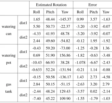
6.1 Estimated absolute rotation of the object and error in degrees . . . 80

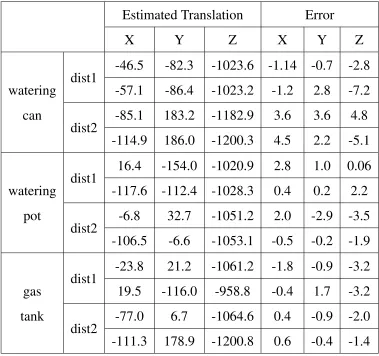
6.2 Estimated absolute translation of the object and error in centimeters . . . 81

6.3 Average precision on the introduced outdoor dataset . . . 81

7.1 Comparison of CNN and HOG-SVM in part localization . . . 89

7.2 Notations in the facility location problem . . . 90

7.3 Model fitting error of PopUp versus FG3D . . . 97

7.4 Coarse viewpoint estimation accuracy versus VDPM . . . 98

7.5 Model sensitivity to the number of shape basis . . . 100

7.6 Model fitting error of PopUp versus FG3D . . . 100

7.7 Average Viewpoint Accuracy on four categories of PASCAL3D . . . 101

8.1 3D reconstruction given 2D poses . . . 119

8.2 Quantitative comparison on Human 3.6M datasets . . . 120

8.3 Quantitative CNN joint error on Human 3.6M datasets . . . 121

8.4 The estimation errors after separate steps and under additional settings . . 122

8.5 Quantitative results on the HumanEva I dataset . . . 125

List of Figures

1 The amazing Kostas’ research group . . . vi

1.1 Overview of the 3D object recognition problem . . . 5

1.2 Active DPM Overview . . . 11

1.3 Overview of the proposed 3D pose estimation of object instances approach 13 1.4 Illustrative summary of single image popup method . . . 15

1.5 Overview of the articulated 3D Pose Estimation approach . . . 16

3.1 GoogleNet: Going Deeper with Convolutions . . . 29

5.1 Active DPM Overview . . . 42

5.2 Score likelihoods for several parts from a car DPM model . . . 47

5.3 Active inference of deformable part models at different locations . . . 52

5.4 Average precision and relative number of part evaluations . . . 54

5.5 Illustration of the ADPM inference process on a car example . . . 57

5.6 Precision recall curves on a subset of PASCAL 2007 . . . 60

6.1 Demonstration of the proposed approach on a PR2 robot platform . . . . 64

6.2 Overview of the proposed approach . . . 64

6.3 Comparison of the two edge detection methods . . . 70

6.4 Spray bottle detection using S-DPM . . . 72

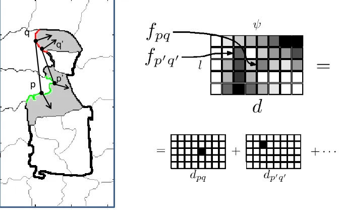
6.5 Chordiogram construction . . . 73

6.6 Shape descriptor-based verification examples . . . 75

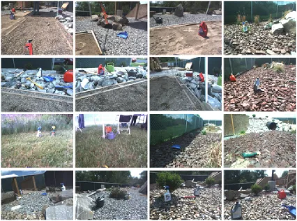
6.7 Representative images from the introduced outdoor dataset . . . 78

7.1 Illustrative summary of single image popup method . . . 84

7.2 Visualization of the optimized landmark selection result. . . 91

7.3 Car type specific meanAPD of PopUp versus FG3D . . . 97

7.4 Continuous viewpoint (azimuth) error on FG3DCar . . . 98

7.5 Precision recall curves for continuous viewpoint estimation . . . 102

7.6 Example 3D estimation results from FG3DCar. . . 104

7.7 Examples of landmark localization results on PASCAL3D . . . 105

8.1 Overview of the proposed approach . . . 107

8.2 Example frame results on Human3.6M . . . 123

8.3 Example results on PennAction. . . 126

8.4 Single image grasping example screen shots . . . 133

8.5 Iterative optimization of the Popup . . . 134

8.6 Iterative optimization of the Popup Continued . . . 135

8.7 Landmark reprojection results on Pascal3D . . . 136

8.8 Landmark reprojection results on Pascal3D, Cont. . . 137

8.9 More example frame activations and results on Human3.6M . . . 138

Part I

Chapter 1

Introduction

There is no royal road to geometry [other than theElements].

— Euclid, on if there is an easier way of learning geometry.

The idea of autonomous robots being able to interact with its surroundings, serving hu-man beings in various tasks, dates back to the ancient Greek mythologies. The depiction of the mechanical servants built by the Greek god Hephaestus is one of the earliest expres-sions of such dream of human kind. This dream has long been fascinating and nowadays extended far beyond the form of mere humanoid robot servants but as autonomous vehi-cles, flying drones, Internet connected devices and smart wearable gadgets, etc. A key component of such intelligent robotic systems lies in their capacities of 3D object recog-nition, i.e., the ability to localize, identify and infer the 3D geometryof massive amount of different objects including us, human, in an unknown environment.

2009;Everingham et al.,2010), the community has harnessed fruitful results as the state of the art in detecting object categories has improved dramatically (Felzenszwalb et al.,

2010b;Girshick et al.,2014).

However, recognition means more than just high precision and recall in detection or classification in 2D. The ultimate goal of recognition is to enable robots to take mean-ingful actions in 3D. Both accuracy, efficiency and the level of details captured by the vision systems are crucial. Firstly, fast and robust object recognition assures the robots to perform tasks reliably in a reasonable amount of time without appearing dumb or over-thinking. In general, there exists a trade-off between efficiency and accuracy, given limited computational resource. It is meaningful to consider striking a balance between these two factors and build a fast system that only tolerances bounded error. Secondly and more importantly, the images are flat but our world is not. It is the reasoning of detailed object 3D geometry that lays the foundation of robotic interactions, such as manipulation, in the real world. The link between 2D and 3D recognition is not yet well established within the community. Designing algorithms that extend beyond recognition in 2D into estimating the 3D information of the objects from images is thus desirable.

Perhaps the most intriguing aspect of the quest is that bridging the gap between 2D and 3D recognition requires more than just learning and matching patterns but jointly reason-ing with the prior knowledge of the 3D world geometry. That draws analogy to the actual human thinking process (Kahneman, 2011), in which both the instinct system – fast and mostly pattern matching – and the logical system – slow but deliberate – work cohesively together for a final decision. The hope here is to peak into the essence of true intelligence following such direction. With all the challenges present and fascinating future awaits, 3D object recognition is a key step to take along the journey towards realizing the dream of intelligent robots.

1.1 Problem Statement

Problem 1(Monocular 3D Object Recognition).

Input: A singleRGBimage orRGBvideo sequence of arbitrary scene. The images could contain arbitrary number of objects including human.

Output: (1) 2D bounding boxes indicating the detected objects and human; (2) 3D ori-entation, translation and surface mesh model of the objects; 3D oriori-entation, trans-lation and skeletal pose of human.

Complexity: Polynomial computational time and space in the number of input pixels and number of output detections and number of object categories.

More specifically, the problem can be split into the following two separate tasks:

• 2D Detection: identify and localize a particular object.

• 3D Recognition: estimate detailed 3D geometric information of the detected objects.

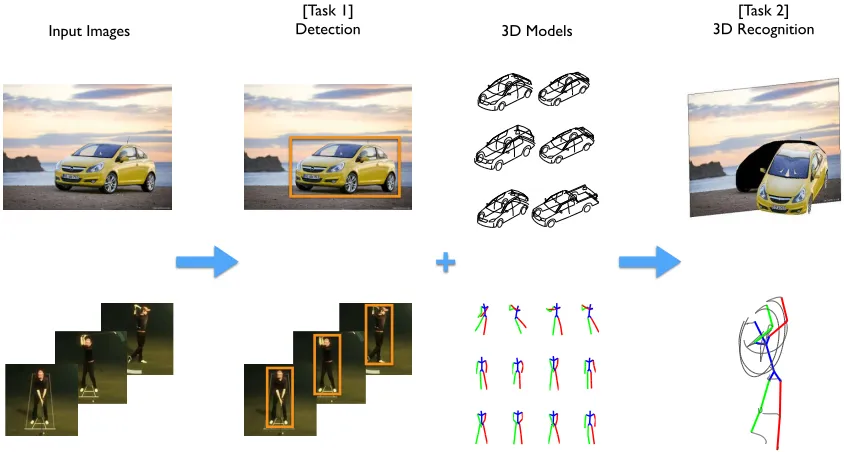
[Task 2] 3D Recognition 3D Models

Input Images

[Task 1] Detection

+

Figure 1.1: Overview of the 3D object recognition problem. Column-wise from left to right: (1) the input image or image sequence; (2) the first task of the problem is to detect the objects and output 2D bounding boxes indicating the location and the scale of the detections; (3) the 3D models of the objects are given; (4) the second task of the problem is to estimate 6-DOF pose and 3D shape mesh model for objects and 3D skeletal pose for human.

1.2 Challenges

The challenges in 3D object recognition can be roughly classified into three categories, namely the appearance variation, depth uncertainty and computational complexity. The appearance variation casts difficulties in localizing and identifying the objects. The depth uncertainty of each pixel is caused by the image formation process itself in which 3D ob-jects are projected into 2D. The lost in depth dimension creates impediments in recovering the original 3D pose and shape of the object. Another challenge lies in the computational complexity as detectors should be efficient enough for real applications. Each challenge is discussed in detail in the following sections.

1.2.1 Appearance Variation

The appearance of an object can be affected by different aspects, such as inter class vari-ation, lightening changes, pose variation etc. In terms of detection the following factors cast the most challenges.

Intra-class differences First, because of the hierarchical structure of object category taxonomy, object instances of the same category may belong to different sub-categories that can appear quite differently. For example, the car category can be further separated into sedan, hatchback, truck etc. The overall shape of a sedan is largely different from that of a truck. Second, even the same object instance can appear drastically different due to changes in lightening, covering material and texture etc. For example, a person wearing different clothings varies a lot in appearance.

rigid template. For non-rigid object such as human, self occlusion cause by the articulation of body pose also changes the appearances.

Background clutter and occlusion The surrounding background of an object can cause trouble in detecting an object. Just imagine playing the game of “Where’s Waldo?”. The presented noisy clutter background overwhelms the presence of the object and usually triggers false positive detections from the detector. An ideal detector should reliably tell the differences between foreground and background. In addition, occlusion by other ob-jects alters the perceived silhouette shape of an object. It is already hard for me to find the red-white-strip shirt of Waldo among the enormous crowd, not to mention when he is partially blocked by someone else!

1.2.2 Depth Uncertainty

The biggest hurdle in 3D object recognition from 2D is the depth uncertainly raised natu-rally from the image formation process. In the classic pinhole camera model, each image coordinate (u, v)is associated with a ray λ(X, Y, Z) in 3D passing through the camera

center, where λ is a the positive unknown scaling factor inverse proportional to depth Z. Here we assume the focal length is f and the radial distortion is not considered for simplicity of discussion. The relation between 2D and 3D can be expressed as

     u v 1     ∼λ     

f 0 0

0 f 0

0 0 1

          X Y Z     .

Non-rigid human pose Comparing to rigid pose and shape estimation problem, recov-ering non-rigid pose or motion from images is more daunting. First, it is challenging to accurately localize the human joints due to the lack of distinctive texture, appearance vari-ation, foreshortening and occlusion, etc. Second, each joint angle in 3D is ambiguous even given the perfectly localized 2D position. Either pointing inwards or outwards can result in the same projection. The lack of the rigidity constrains makes the problem much harder to solve.

1.2.3 Computational Issues

Computational complexity is another practical concern of the object recognition algo-rithms. Both the learning and inference algorithms should complete within a reasonable amount of computational time and space. Both the model and algorithmic complexity require careful design.

Efficiency and accuracy When dealing with 2D object detection task, a sliding window approach is usually adopted. The detector searches over the entire 2D image location and scale space, or the image pyramid. Each location is examined one after another with an object specific classifier to see if there exists an object or not. The computational time of such approach grows as the time for evaluating each classifier increases. This approach becomes more computationally intense as the classifier requires more processing time. On the other hand, better recognition accuracy is usually achieved with more sophisticated model which requires longer time to evaluate. The challenge here is to strike a balance between the efficiency and accuracy.

Search over rotations The 3D pose estimation problem encompasses a parameter search space over the 3D rotation groupSO(3). SO(3) is the special orographic orthogonal in

One would either follow the geodesic on the manifold from certain initialization or resort to an exhaustive search approach. The former approach suffers poor initialization and the latter has difficulties in handling practical problems as the exhaustive search is too time consuming.

Search over instances In the task of 3D shape estimation, recovering an accurate shape is relatively easy when the instance is known. In that case, the shape estimation problem is reduced to a nearest neighbor problem given the database of known instance. The most trivial approach means searching over all the instances of an object category to find the matching one. Linearly searching over the models can be very inefficient and quickly becomes infeasible for practical problems. Therefore the model representation should be compact, i.e. sub-linear or even constant w.r.t. the number of instances, and still represent the entire object category. However, if the instance is unknown or not exactly covered by the model database, estimating the accurate shape is quite challenging.

1.3 Contributions

Deformable part model (DPM) (Felzenszwalb et al., 2010c), arguably one of the most successful object detectors in the past decade, represents the object as a union of parts connected in a star structure.DPM and its variants achieved the state-of-art object detec-tion results on the most popular object recognidetec-tion benchmarks such as PASCAL VOC (Everingham et al.,2010) and ImageNet (Deng et al.,2009). The key to such success lies in the combination between rigid parts and 2D deformation. The part appearances learned from data are discriminative enough to handle intra-class variation and the 2D deformation of the parts allow flexibility to deal with inter-class variation.

There have been several directions to which the researchers extended the powerful DPM models. One is to accelerate the detection process of DPM. By incorporating the idea of cascade (Doll´ar et al.,2012;Felzenszwalb et al.,2010a;Sapp et al.,2010;Weiss et al.,

to actually evaluate the full model during inference; Another is to increase the model complexity to deal with structured output problems other than the binary classification problem as usually presented in object detection. For example, more parts are added to form a tree-structure model for human pose estimation (Yang and Ramanan, 2011) or facial landmarks localization (Zhu and Ramanan,2012); Generic 3D object recognition is pioneered bySavarese and Fei-Fei (2007). More recently, researchers have been focused on combining part models with 3D geometry to build more powerful object detectors that are also able to provide 3D information such as viewpoint (Hu and Zhu, 2014; Liebelt et al.,2008b;Pepik et al.,2012b,c;Zia et al.,2013). Few efforts have been devoted to the combined estimation of pose and shape from a single image (Hejrati and Ramanan,2012;

Lin et al.,2014;Xiang and Savarese,2012).

This thesis advances the start-of-art in the following two directions.

First, the proposed Active Deformable Part Models (ADPM) pushes the DPM accel-eration further by considering part evaluation as aplanning problem. An active inference process decides at each image location whether to evaluate more parts and in what order or to stop and predict a label. A policy is learned off-line to balance the trade-off between the acceleration gain and detection accuracy loss across the entire training set. The result pol-icy leads to a three times speed-up versus the prior work of Cascade DPM (Felzenszwalb et al.,2010a).

Figure 1.2:Active DPM Overview: A deformable part model is shown with colored root and parts in the first column. The second column contains an input image and the original DPM scores as a baseline. The rest of the columns illustrate the inference process of the Active DPM, which proceeds in rounds. The foreground probability is maintained at each image location (top row) and is updated sequentially. A policy (learned off-line) is used to select the best sequence of parts to apply at different locations. The bottom row shows the part filters applied at consecutive rounds with colors corresponding to the parts on the left. For more detailed explanation, see§5

1.3.1 Efficient 2D Object Detection,

§

5

Active Deformable Part Models (ADPM), named so because of the active part selection. The detection procedure consists of two phases: an off-line phase, which learns a part scheduling policy from the training data and an online phase (inference), which uses the policy to optimize the detection task on test images. During inference, each image location starts with equal probabilities for object and background. The probabilities are updated sequentially based on the responses of the part filters suggested by the policy. At any time, depending on the probabilities, the policy might terminate predicting either a background label (which is what most cascaded methods take advantage of) or a positive label, in which case all unused part filters are evaluated in order to obtain the complete DPM score. Fig. 1.2exemplifies the inference process. The main contributions can be summarized as the following:

• We obtain an active part selection policy which optimizes the order of the filter

evaluations and balances number of evaluations used with the classification accuracy based on the scores obtained during inference.

• The proposed detector achieves a significant speed-up versus the cascade DPM

with-out sacrificing accuracy.

• The approach can be generalized to any detection problem, which involves a linear additive score and uses several parts (stages) even if they are just SIFT points.

1.3.2 3D Pose Estimation of Object Instances,

§

6

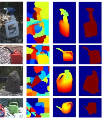
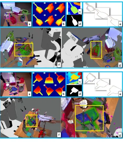
Figure 1.3: Overview of the proposed 3D pose estimation of object instances approach. From left-to-right: a) The input image. b) S-DPM detection hypothesis on the image contours. c) The hypothesis bounding box (red) is segmented into superpixels. d) The set of superpixels with the closest chordiogram distance to the model silhouette is selected. Pose is iteratively refined such that the model projection aligns well with the foreground mask silhouette. e) Three textured synthetic views of the final pose estimate are shown.

Object silhouettes with corresponding viewpoints that are tightly clustered on the viewsphere are used as positive exemplars to train the state-of-the-art Deformable Parts Model (DPM) (Felzenszwalb et al., 2010c). We term this shape-aware version S-DPM. S-DPM simultaneously detects the object and coarsely estimates the object’s pose. We propose to apply an S-DPM classifier on image contours as a first high recall step yield-ing several boundyield-ing box hypotheses. Given these hypotheses, we solve for segmentation and localization simultaneously. After over-segmenting the hypothesis region into super-pixels, the superpixels that best match a model boundary are selected using a shape-based descriptor, the chordiogram (Toshev et al.,2012). A chordiogram-based matching distance is used to compute the foreground segment and rerank the hypotheses. Finally, using the full 3D model we estimate all 6-DOF of the object by efficiently iterating on the pose and computing matches using dynamic programming.

robot operation, where popular RGB-D sensors cannot be used (e.g., outdoors) and stereo sensors are challenged by the uniformity of the object’s appearance within their boundary. Fig. 1.3exemplifies the inference process. The main contributions can be summarized as the following.

• In terms of assumptions, our approach is among the few in the literature that can

detect 3D objects in single images of cluttered scenes independent of their appear-ance.

• It combines the high recall of an existing discriminative classifier with the high precision of a holistic shape descriptor achieving a simultaneous segmentation and detection reranking.

• Due to the segmentation, it selects the correct image contours to use for 3D pose refinement, a task that was previously only possible with stereo or depth sensors.

1.3.3 3D Pose and Shape Estimation of Object Categories,

§

7

We propose a novel approach that marries the power of discriminative parts with an ex-plicit 3D geometric representation with the goal to infer 3D shape and continuous pose of an object (orpop-up) from a single image. Part descriptors are discriminatively learned in training images. Such parts are centered around projections of 3D landmarks which are given in abundance on the training 3D models. To establish a compact representation we minimize the number of needed landmarks by solving a facility-location problem.

+ =

3D Shape Constrained

Discriminative Parts 3D Shape Space + Detection HypothesesIndividual Part Pop-Up !

Figure 1.4: Illustrative summary of the single image popup approach: 3D Landmarks on a 3D model are associated with discriminatively learned part descriptors (left). Intra-class shape variation is captured with linear combinations of a sparse shape basis (2nd left). Learned part descriptors produce multiple maximum responses for each part in a testing image (3rd from left). The selection of the part hypotheses, 3D pose and 3D shape are simultaneously estimated and the result is illustrated through a popup (right).

pose parameters in one step using a convex program solved with the alternating direction method of multipliers (ADMM). Fig. 1.4 exemplifies the inference process. The main contributions can be summarized as the following.

• A convex optimization framework for joint landmark localization, fine grained 3D

shape and continuous pose estimation from a single image.

• Our convex objective does not require viewpoint or detection initialization.

• An automatic landmark selection method considering both discriminative power in

appearance and spatial coverage in geometry.

1.3.4 Articulated 3D Pose Estimation from Image Sequences,

§

8

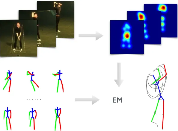
EM

……

Figure 1.5: Overview of the proposed articulated 3D Pose Estimation approach. (top-left) Input image sequence, (top-right) CNN-based heat map outputs representing the soft lo-calization of 2D joints, (bottom-left) 3D pose dictionary, and (bottom-right) the recovered 3D pose sequence reconstruction.

include human-computer interaction (cf. (Shotton et al.,2011)), surveillance, video brows-ing and indexbrows-ing, and virtual reality.

A 3D pose recovery framework that consists of a novel synthesis between discrim-inative image-based and 3D reconstruction approaches is presented. In particular, the approach reasons jointly about image-based 2D part location estimates and model-based 3D pose reconstruction, so that they can benefit from each other. Further, to improve the approach’s robustness against detector error, occlusion, and reconstruction ambiguity, temporal smoothness is imposed on the 3D pose and viewpoint parameters.

relaxing the common but restrictive assumption that the 2D poses are provided or explic-itly estimated (cf. (Wang et al.,2014)) and instead treats the 2D pose as a latent variable. A CNN-based body joint detector is used to learn the uncertainty map for the image location of each joint. To estimate the 3D pose, an efficient EM algorithm is proposed, where the latent joint positions are marginalized to fully account for the uncertainty in the 2D joint locations. Finally, empirical evaluation demonstrates that the proposed approaches are more accurate compared to extant approaches. In particular, in the case where 2D joint locations are provided, the proposed approach exceeds the accuracy of the state-of-the-art NRSFM baseline (Dai et al.,2012) on the Human3.6M dataset (Ionescu et al., 2014). In the case where the 2D landmarks are unknown, empirical results on the Human3.6M dataset demonstrate overall improvement over published results. Further, the proposed approach is shown to outperform a publicly available 2D pose estimation baseline on the challenging PennAction dataset (Zhang et al., 2013). Fig. 1.5 exemplifies the inference process.

1.3.5 Published Work Supporting This Thesis

Active Deformable Part Models (§5) is presented in (Zhu et al., 2014a) for fast object detection. Single Image 3D Object Pose Estimation (§6) first appeared in (Zhu et al.,

2014b) that enables robots grasping different objects by only taking a single image of the scene. The method of 3D pop-up from single images (§7) extended the scope of single

Chapter 2

Related Work

2.1 Accelerated Object Detection

We will refer to work on object detection that optimizes the inference stage rather than the representations since our representation is identical with DPM (Felzenszwalb et al.,

detectors based on a sliding window or a Hough transform but without deformable parts. Another related group of approaches focuses on learning a sequence of object template tests in position, scale, and orientation space that minimizes the total computation time through a coarse-to-fine evaluation (Fleuret and Geman,2001;Pedersoli et al.,2011).

The classic work by Viola and Jones (Viola and Jones, 2001) introduced a cascade of classifiers whose order was determined by importance weights learned by AdaBoost. The approach was studied extensively in (Bourdev and Brandt, 2005; Brubaker et al., 2008;

Gualdi et al., 2012; Lehmann et al., 2011a; Zhang et al., 2011). Recently, Dollar et al. (Doll´ar et al.,2012) introduced cross-talk cascades which allow detector responses to trig-ger or suppress the evaluation of weak classifiers in their neighborhood by exploiting the correlation of the classifier responses in the neighboring positions and scales. Weiss et al. (Weiss et al., 2012) used structured prediction cascades to optimize a function with two objectives: pose refinement and minimum filter evaluation cost. Sapp et al. (Sapp et al.,2010) learn a cascade of pictorial structures with increasing pose resolution by pro-gressively filtering the pose state space. Its emphasis is on pre-filtering structures through max-margin scoring rather than part locations so that human poses with weak individ-ual part appearances can still be recovered. Rahtu et al. (Rahtu et al., 2011) use general “objectness” filters to produce location proposals which are fed into a cascade, designed to maximize the quality of the locations that advance to the next stage. Our approach is also related to and could be combined with active learning using Gaussian processes for classification (Kapoor et al.,2010).

Similarly to the closest approaches above (Felzenszwalb et al.,2010a;Kokkinos,2011;

2.2 Rigid Object Pose Estimation

Early approaches based on using explicit 3D models are summarized in Grimson’s book (Grimson,1990) and focus on efficient techniques for voting in pose space. Horaud ( Ho-raud,1987) investigated object recognition under perspective projection using a construc-tive algorithm for objects that contain straight contours and planar faces. Hausler (H¨ausler and Ritter,1999) derived an analytical method for alignment under perspective projection using the Hough transform and global geometric constraints. Aspect graphs in their strict mathematical definition (each node sees the same set of singularities) were not considered practical enough for recognition tasks but the notion of sampling of the view-space for the purpose of recognition was introduced again in (Cyr and Kimia, 2001) which were applied in single images with no background. A Bayesian method for 3D reconstruction from a single image was proposed based on the contours of objects with sharp surface in-tersections (Han and Zhu,2003). Sethi et al. (Sethi et al.,2004) compute global invariant signatures for each object from its silhouette under weak perspective projection. This ap-proach was later extended (Lazebnik et al., 2002) to perspective projection by sampling a large set of epipoles for each image to account for a range of potential viewpoints. Liebelt et al. work with a view space of rendered models in (Liebelt et al., 2008a) and a genera-tive geometry representation is developed in (Liebelt and Schmid,2010). Villamizar et al. (Villamizar et al., 2011) use a shared feature database that creates pose hypotheses veri-fied by a Random Fern pose specific classifier. In (Glasner et al.,2011a), a 3D point cloud model is extracted from multiple view exemplars for clustering pose specific appearance features. Others extend deformable part models to combine viewpoint estimates and 3D parts consistent across viewpoints, e.g., (Pepik et al.,2012a). In (Hao et al.,2013), a novel combination of local and global geometric cues was used to filter 2D image to 3D model correspondences.

shapes and a two-step iteration optimizes over shape and pose, respectively (Prisacariu et al., 2013). The drawback of these approaches is that in the case of scene clutter they do not consider the selection of image contours. Further, in some cases tracking is used for finding the correct shape. This limits applicability to the analysis of image sequences, rather than a single image, as is the focus in the current paper.

Our approach resembles early proposals that avoid appearance cues and uses only the silhouette boundary, e.g., (Cyr and Kimia, 2001). None of the above or the exemplar-based approaches surveyed below address the amount of clutter considered here and in most cases the object of interest occupies a significant portion of the field of view.

Early view exemplar-based approaches typically assume an orthographic projection model that simplifies the analysis. Ullman (Ullman and Basri, 1991) represented a 3D object by a linear combination of a small number of images enabling an alignment of the unknown object with a model by computing the coefficients of the linear combination, and, thus, reducing the problem to 2D. In (Basri,1993), this approach was generalized to objects bounded by smooth surfaces, under orthographic projection, based on the estima-tion of curvature from three or five images. Much of the multiview object detector work based on discrete 2D views (e.g., (Gu and Ren, 2010a)) has been founded on successful approaches to single view object detection, e.g., (Felzenszwalb et al., 2010c). Savarese and Fei-FeiSavarese and Fei-Fei (2007) presented an approach for object categorization that combines appearance-based descriptors including the canonical view for each part, and transformations between parts. This approach reasons about 3D surfaces based on image appearance features. In (Payet and Todorovic,2011), detection is achieved simulta-neously with contour and pose selection using convex relaxation. Hsiao et al. (Hsiao et al.,

As far as RGB-D training and test examples are concerned, the most general and rep-resentative approach is (Lai et al.,2011). Here, an object-pose tree structure was proposed that simultaneously detects and selects the correct object category and instance, and refines the pose. In (Rusu et al., 2010), a viewpoint feature histogram is proposed for detection and pose estimation. Several similar representations are now available in the Point Cloud Library (PCL) (Rusu and Cousins, 2011). We will not delve here into approaches that extract the target objects during scene parsing in RGB-D images but refer the reader to (Koppula et al.,2011) and the citations therein.

The 2D-shape descriptor, chordiogram (Toshev et al., 2012), we use belongs to ap-proaches based on the optimal assembly of image regions. Given an over-segmented image (i.e., superpixels), these approaches determine a subset of spatially contiguous re-gions whose collective shape (Toshev et al., 2012) or appearance (Vijayanarasimhan and Grauman,2011) features optimize a particular similarity measure with respect to a given object model. An appealing property of region-based methods is that they specify the im-age domain where the object-related features are computed and thus avoid contaminating objected-related measurements from background clutter.

2.3 3D Shape Reconstruction

(Hejrati and Ramanan,2012;Hu and Zhu,2014;Lin et al.,2014;Zia et al.,2013) and hu-man pose estimation (Ramakrishna et al.,2012;Zhou and De la Torre,2014). Our method differs in that we use a data-driven approach for discriminative landmark selection and we solve landmark localization and shape reconstruction in a single convex framework, which enables a global solution.

The representation of our model is inspired by recent advances in part-based modeling (Felzenszwalb et al., 2010b;Hariharan et al.,2012; Kokkinos,2011;Singh et al., 2012), which models the appearance of object classes with a collection of mid-sized discrimi-native parts. Our optimization approach is related to the previous work on using convex relaxation techniques for object matching (Jiang et al., 2011;Li et al., 2011;Maciel and Costeira, 2003). These methods focused on finding the point-to-point correspondence between an object template and an image in 2D, while our method considers 3D to 2D matching as well as shape variability.

Our paper is also related to recent work on 3D pose estimation which encodes the geometric relations among local parts and achieved continuous pose estimation. Several work leveraged 3D models to warp features or parts into their canonical view (Savarese and Li, 2007; Xiang and Savarese, 2012; Yan et al., 2007). Other work rendered local appearances and depth from 3D models and subsequently encoded in a 3D voting scheme (Glasner et al., 2011b; Liebelt et al., 2008b; Sun et al., 2010). DPM was further lifted to 3D deformable models (Fidler et al., 2012; Pepik et al., 2012b) to predict continuous viewpoint. Instance models were also used to recover 3D pose of an object (Aubry et al.,

2.4 Articulated 3D Pose Estimation

Considerable research has addressed the challenge of 3D human motion capture from video (Brubaker et al.,2010;Moeslund et al.,2006;Sminchisescu,2007). Early research on 3D monocular pose estimation in videos largely centred on incremental frame-to-frame pose tracking, e.g., (Bregler and Malik,1998;Sigal et al.,2012;Sminchisescu and Triggs,

2003). These approaches rely on a given pose and dynamic model to constrain the pose search space. Notable drawbacks of this approach include: the requirement that the initial-ization be provided and their inability to recover from tracking failures. To address these limitations, more recent approaches have cast the tracking problem as one of data asso-ciation across frames, i.e., “tracking-by-detection”, e.g., (Andriluka et al., 2010). Here, candidate poses are first detected in each frame and subsequently a linking process at-tempts to establish temporally consistent poses.

Another strand of research has focused on methods that predict 3D poses by searching a database of exemplars (Jiang,2010;Mori and Malik,2006;Shakhnarovich et al.,2003) or via a discriminatively learned mapping from the image directly or image features to human joint locations (Agarwal and Triggs, 2006; Ionescu et al., 2014; Salzmann and Urtasun,2010;Tekin et al.,2015;Yu et al.,2013). Recently, deep convolutional networks (CNNs) have emerged as a common element behind many state-of-the-art approaches, including human pose estimation, e.g.,Li and Chan(2014);Li et al.(2015);Tompson et al.

(2014);Toshev and Szegedy(2014). Here, two general approaches can be distinguished. The first approach casts the pose estimation task as a joint location regression problem from the input image (Li and Chan,2014;Li et al.,2015;Toshev and Szegedy,2014). The second approach uses a CNN architecture for body part detection (Chen and Yuille,2014;

Jain et al., 2014; Pfister et al., 2015; Tompson et al., 2014) and then typically enforces the 2D spatial relationship between body parts as a subsequent processing step. Similar to the latter approaches, the proposed approach uses a CNN-based architecture to regress confidence heat maps of 2D joint position predictions.

recovering 3D non-rigid shapes from image sequences captured with a single camera (Akhter et al., 2011; Bregler et al., 2000; Cho et al., 2015; Dai et al., 2012; Zhu et al.,

2014c), i.e., non-rigid structure from motion (NRSFM), and human pose recovery models based on known skeletons (Lee and Chen, 1985; Park and Sheikh, 2011; Taylor, 2000;

Valmadre and Lucey,2010) or sparse representations (Akhter and Black,2015;Fan et al.,

2014;Ramakrishna et al., 2012;Zhou et al., 2015b,c). Much of this work has been real-ized by assuming manually labeled 2D joint locations; however, there is some recent work that has used a 2D pose detector to automatically provide the input joints (Wang et al.,

Part II

Chapter 3

Discriminative Learning

In this chapter, we briefly cover the basics of discriminative learning and introduce two successful methods on which this thesis is based.

In the machine learning literature, classifiers generally fall into two categories: gener-ative classifiers and discrimingener-ative classifiers. Genergener-ative classifiers learn the joint distri-butionp(y, x)of the inputxand the labely. Combined with the prior distributionp(x)of

the label, the posterior distributionp(y_|x)is then derived using Bayes rules.

Discrimina-tive classifiers learn the posterior distributionp(y_|x)directly by modeling the distribution

with a parametric model and optimizes the parameters using a training set. In the seminal work of (Ng and Jordan, 2002), the two types of classifiers are compared and the results suggest that discriminative models have lower asymptotic error given large training data.

3.1 Support Vector Machine

One particularly successful discriminative model is Support Vector Machine (SVM), with many applications to document classification, object classification etc. SVM was orig-inally started when statistical learning theory was developed further by Vapnik (Vapnik and Kotz, 1982) and later extended closer to its current form (Cortes and Vapnik, 1995). For simplicity, we only discuss the linear SVM. The non-linear SVM extends the linear case and builds on the idea of kernel methods, which is out of the scope of this thesis.

The linear SVM learns a separating hyperplane wT_{x+b = 0from labeled examples}

D =_{hx1, y1i, ...,hxn, yni}, whereyi ∈ {−1,1}. In order to achieve robustness to noise

and gain better generalization to unseen data, SVM maximizes the margin of the separating hyperplane to the examples. Formally, linear SVM can be formulated as the following optimization problem,

min

w,b,ξ≥0

1 2w

T

w+CX

i

ξi (3.1)

s.t. yi(wTxi+b)≥1−ξi, i= 1, ..., n, (3.2)

where ξi is called the slack variable, introduced for penalizing the incorrectly classified

examples,C is the weight on the penalty cost.

By taking the gradient w.r.t. wandbon the corresponding Lagrangian, we can derive the equivalent dual problem as,

max

α≥0

X

i

αi−

1

2αiαjyiyjx

T

ixi (3.3)

s.t. X

i

αiyi = 0, αi ≤C, i= 1, ..., n, (3.4)

where αi is the Lagrange multiplier for the inequality constrain 3.2 in the primal form.

Figure 3.1: GoogleNet desgined by (Szegedy et al., 2015): an example of modern deep convolutional neural network with many layers of convolutions, where the blue boxes are the convolution layers.

to tackle the problem, and we refer curious readers to an excellent tutorial by Burges

(1998) for more details.

3.2 Deep Neural Networks

The development of neural networks dates back to 1957 when Frank Rosenblatt invented a linear classifier called the perceptron (Rosenblatt,1961). One of the early success of neu-ral networks was when convolutional neuneu-ral networks (LeCun et al., 1989) was invented and successfully applied to handwritten digit recognition in the 90s. After the initial hype the related research went mostly under the radar of the computer vision community par-tially due to the success of SVMs. Until recently, with the advances of computing hard-ware especially Graphics Processing Units (GPU), convolutional neural netwroks staged a huge comeback after winning the 2012 ImageNet Challenge (Krizhevsky et al., 2012). Interestingly, despite the differences of modern deep learning models with many more lay-ers3.1 than their predecessors, the learning algorithm of the neural networks has remain the same, namely back-propagationRumelhart et al.(1988).

function of the layer that precedes it. In this structure, the each layer i _{∈ {}1, ..., n_} is given by

h(i)=g(i)(W(i)Th(i−1)+b(i)) (3.5)

whereh(i)_{is the activation of each layer andh}(0) _{=xis the input data. Note in the case of}

convolutional neural network, convolutions can be rearranged as matrix multiplications. g(i) _{is a nonlinear function applied after the linear transform of the activations from the}

previous layer. The choice of nonlinear activation functions can be Rectified Linear Units (ReLU), logistic, max pooling etc.

The universal approximation theorem (Hornik et al.,1989) states that under mild as-sumptions on the activation mapping, neural networks with a single hidden layers can approximate continuous functions on compact sets of Rn_{. Modern multi-layered deep}

neural networks have much bigger capacity but the nonlinearity still poses a big challenge to learning such complex model.

In general, the cost function of a network is a non-convex function w.r.t. to input, thus learning the parameters of a neural network is usually resorted to gradient decent. The minimization of the cost function is generally carried out via error back-propagation (Rumelhart et al.,1988), or in other words, propagating the gradients using the chain rule. More specifically, the following derivation

∂h(n)

∂h(i) =

∂h(n)

∂h(n−1)

∂h(n−1)

∂h(i) (3.6)

3.3 Stochastic Gradient Descent

The robustness of discriminative classifiers generally improves as more training examples are exposed. However, as the datasets grow larger in scale, parameter learning with gra-dient descent via batch optimization usually cannot be directly applied due to machine memory limitations and computational efficiency reasons. In such cases, stochastic gra-dient descent is deployed iteratively to approximate the gragra-dient that would be computed from the whole dataset.

In general, the learning algorithm minimizes the sum of empirical losses over a dataset, more specifically an objective function of the form,

J(θ) =

n

X

i=1

Ji(θ), (3.7)

whereθis the parameter to be estimated. A standard batch gradient descent method would updateθas the following,

θ=θ₋η

n

X

i=1

∇Ji(θ) (3.8)

With stochastic gradient descent, the batch gradient is approximated with the gradient at a single example,

θ =θ₋η_∇Ji(θ). (3.9)

Chapter 4

Convex Optimization

In this chapter, we discuss a class of optimization methods that are most related to this thesis called Proximal Algorithms. This class of optimization algorithms are designed for challenges raise in constrained convex optimization problems with non-smooth objective function. First, we discuss the general concepts and underlying theory of Proximal Al-gorithms. Then we focus our discussion on a powerful subclass: Alternating Direction Method of Multipliers.

4.1 Proximal Algorithms

4.1.1 Proximal Operator

Definition 1. The proximal operator prox_f :Rn_→Rnoff is defined by prox_f(v) = arg min

x

f(x) + (1/2)_kx₋v_k2₂. (4.1) The function minimized on the right-hand side is strongly convex w.r.t. v and not every-where infinite, so it has a unique minimizer for everyv _∈Rn_.

The proximal operator of the scaled functionλf, whereλ >0, is expressed as

proxλf(v) = arg min x

f(x) + (1/2λ)_kx₋v_k2₂. (4.2)

Proposition 1. The pointx∗ minimizesf if and only if x∗ =prox_f(x∗), i.e., ifx∗ is a fixed point of prox_f.

This fundamental property gives a link between proximal operators and fixed point theory;e.g., many proximal algorithms for optimization can be interpreted as methods for finding fixed points of appropriate operators. For the proof of the proposition we refer to (Parikh and Boyd,2013).

4.1.2 Moreau Decomposition

The convex conjugate (Boyd and Vandenberghe,2004) of a functionf is defined as, f∗(y) = sup

x

yTx₋f(x). (4.3) The following equality always holds:

v =prox_f(v) +prox_f∗(v) (4.4)

This property, known asMoreau decompositiongives a simple way to obtain the proximal operator of a functionf in terms of the proximal operator off∗. For example, iff =_{k · k}

is a general norm, thenf∗ =IB, where

is the unit ball of the dual normk · k∗, defined by

kz_k∗ = sup{zTx| kxk ≤1}.

By Morean decomposition, this implies that

v =prox_f(v) + ΠB(v). (4.5)

We can see that, evaluating proxf(v)is easy if we know how to project one toB.

4.1.3 Proximal Operator of the Spectral Norm

Part of this thesis regarding 3D reconstruction from single image builds on the following proposition (Zhou et al.,2015c) which states the proximal operator of the spectral norm.

Proposition 2. The solution to the following problem

min X

1

2kY−Xk

2

F +λkXk2 (4.6)

is given byX∗ =_Dλ(Y), where

Dλ(Y) = UY diag[σY−λPl1(σY/λ)]V

T

Y, (4.7)

UY, VY and σY denote the left singluar vectors, right singular vectors and singular

values ofY, respectively. _Pl1 is the projection of a vector to the unitl1-norm ball.

Proof The problem in (4.6) is a proximal problem. The associated proximal operator is the solution to the following minimization problem

proxλF(Y) = arg min

X 1

2kY−Xk

2

F +λF(X). (4.8)

In this case,F(X) = _kX_k2 =kσXk∞, where k · k∞ denotes thel∞-norm. Based on the

property of spectral functions (Parikh and Boyd,2013), we have

wheref is thel∞-norm. The poximal operator of thel∞-norm can be computed by

Meo-reau decomposition§4.1.2:

proxλf(σY) =σY−λPl1(σY/λ), (4.10) given that thel1-norm is the dual norm of thel∞-norm.

4.1.4 Proximal Gradient Descent

Consider a general problem of the form

min

x f(x) +g(x), (4.11)

where f : Rn _{→ R and g : R}n _{→ R∪ {+∞} are closed proper convex and f is}

differentiable. The optimality condition is satisfied whenx∗ minimizes4.11such that the following equivalent statements hold for any fixed scalarλ >0

0_∈λ_∇f(x∗) +λ∂g(x∗),

0_∈λ_∇f(x∗)₋x∗+x∗+λ∂g(x∗),

(I+λ∂g)(x∗)_∈(I₋λ_∇f)(x∗),

x∗ = (I+λ∂g)−1(I₋λ_∇f)(x∗). (4.12) Equation4.12leads to an fixed point iterative update scheme:

xk = (I+λ∂g)−1(I−λ∇f)(xk−1), (λ >0) (4.13)

which is equivalent to

xk=proxλg(xk−1−λ∇f(xk−1)) (4.14)

4.2 Alternating Direction Method of Multipliers

solves for the saddle point of the augmented Lagrangian associated with the constrained optimization problem. ADMM has a rather long history in optimzation but recently rec-ognized as a powerful tool to solve many non-smooth, constrained and large scale opti-mization problem. ADMM is also known as Split Bregman method (Goldstein and Osher,

2009).

ADMM solves problems in the form

min

x,z f(x) +g(z)

s.t.Ax+Bz =c.

(4.15)

with variablesx _∈ Rnandz _∈ Rm, where A _∈Rp×n, B _∈ Rp×m, and c_∈ Rp. Both f andg are assumed to be convex.

4.2.1 Augmented Lagrangian

Consider the following problem

min

x f(x)

s.t.Ax=b,

(4.16)

with variablex_∈ Rn_{, whereA ∈ R}m×n_{andf :R}n _{→ Ris convex. The Lagrangian of}

problem (4.16) is

L(x, y) = f(x) +yT(Ax₋b). Now let us look at an equivalent problem

min

x f(x) +

ρ

2kAx−bk

2 2

s.t.Ax=b.

(4.17)

The equivalence is clear since for any feasiblex, the added(ρ/2)_kAx₋b_k2₂term is always zero. The associated Lagrangian

Lρ(x, y) =f(x) +yT(Ax−b) +

ρ

2kAx−bk

2

2. (4.18)

4.2.2 Alternating Direction Minimization

The augmented Lagrangian associated with the problem (4.15) is Lρ(x, z, y) = f(x) +g(z) +yT(Ax+Bz −z) +

ρ

2kAx+Bz −ck

2 2.

ADMM minimizes the objective function by alternatively optimizing the augmented Lagrangian with respect to variablexandzwith method of multipliers. Formally, ADMM consists of the following iterations

xk+1 := arg min

x

Lρ(x, zk, yk) (4.19)

zk+1 := arg min

z

Lρ(xk+1, z, yk) (4.20)

yk+1 :=yk+ρ(Axk+1+Bzk+1₋c), (4.21) whereρ > 0. The algorithm consists of anx-minimization step (4.19)), az-minimization step (4.20), and a dual variable update (4.21). The step size of dual update is equal to the augmented Lagrangian parameterρ.

ADMM is a class of proximal algorithm because the x-update step (4.19) and thez -update step (4.20) is closely related to the proximal update off andg. For simplicity, let us consider the case whenA=I, B=I andc= 0. Then the problem reduced to

min

x,z f(x) +g(z)

s.t.x₋z = 0.

(4.22)

The associated augmented Lagrangian is

Lρ(x, z, y) = f(x) +g(z) +yT(x−z) +

ρ

2kx−zk

2 2.

Then the corresponding ADMM iteration can be expressed as

xk+1 :=prox_λf(zk₋uk) (4.23)

zk+1 :=prox_λg(xk+1+uk) (4.24)

Convergence Under rather mild assumptions: 1) Function f and g are closed, proper and convex; 2) The unaugmented LagrangianL0has a saddle point; The ADMM iterations

satisfy the following:

• Residual convergence.rk _{→0ask→ ∞,i.e.,the iterates approach feasibility.}

• Objective convergence. f(xk) +g(xk)_→p∗ ask _{→ ∞},i.e.,the objective function of the iterates approaches the optimal value.

Part III

Chapter 5

Active Deformable Part Models

5.1 Introduction

Part-based models such as deformable part models (DPM) Felzenszwalb et al. (2010b) have become the state of the art in today’s object detection methods. They offer powerful representations which can be learned from annotated datasets and capture both the appear-ance and the configuration of the parts. DPM-based detectors achieve unrivaled accuracy on standard datasets but their computational demand is high since it is proportional to the number of parts in the model and the number of locations at which to evaluate the part fil-ters. Approaches for speeding-up the DPM inference such as cascades, branch-and-bound, and multi-resolution schemes, use the responses obtained from initial part-location evalu-ations to reduce the future computation. This paper introduces two novel ideas, which are missing in the state-of-the-art methods for speeding up DPM inference.

provides maximal classification accuracy at each location. Our second idea is to use a decision loss in the optimization, which quantifies the trade-off between false positive and false negative mistakes, instead of the threshold-based stopping criterion utilized by most other approaches. These ideas have enabled us to propose a novel object detector, Active Deformable Part Models, named so because of the active part selection. The detection procedure consists of two phases: an off-line phase, which learns a part scheduling policy from the training data and an online phase (inference), which uses the policy to optimize the detection task on test images. During inference, each image location starts with equal probabilities for object and background. The probabilities are updated sequentially based on the responses of the part filters suggested by the policy. At any time, depending on the probabilities, the policy might terminate predicting either a background label (which is what most cascaded methods take advantage of) or a positive label, in which case all unused part filters are evaluated in order to obtain the complete DPM score. Fig. 5.1 exemplifies the inference process.

We evaluated our approach on the PASCAL VOC 2007 and 2010 datasetsEveringham et al. (2010) and achieved state of the art accuracy but with a 7 times reduction in the number of part-location evaluations and an average speed-up of 3 times compared to the cascade DPMFelzenszwalb et al.(2010a). This paper makes the followingcontributions

to the state of the art in part-based object detection:

1. We obtain an active part selection policy which optimizes the order of the filter evaluations and balances number of evaluations used with the classification accuracy based on the scores obtained during inference.

2. The proposed detector achieves a significant speed-up versus the cascade DPM with-out sacrificing accuracy.

Figure 5.1: Active DPM Overview: A deformable part model trained on the PASCAL VOC 2007 horse class is shown with colored root and parts in the first column. The second column contains an input image and the original DPM scores as a baseline. The rest of the columns illustrate the inference process of the Active DPM, which proceeds in rounds. The foreground probability (of a horse being present) is maintained at each image location (top row) and is updated sequentially based on the responses of the part filters (high values are red; low values are blue). A policy (learned off-line) is used to select the best sequence of parts to apply at different locations. The bottom row shows the part filters applied at consecutive rounds with colors corresponding to the parts on the left. The policy decides to stop the inference at each location based on the confidence of foreground. As a result, the complete sequence of part filters is evaluated at very few locations, leading to a significant speed-up versus the traditional DPM inference. Our experiments show that the accuracy remains unaffected.

5.2 Related Work

We will refer to work on object detection that optimizes the inference stage rather than the representations since our representation is identical with DPM (Felzenszwalb et al.,

in the cascade DPM is pre-defined and a set of thresholds has to be determined empiri-cally, our approach selects the part order and the stopping time at each location based on an optimization criterion. We find the next closest approach to be (Sznitman et al.,2013), which maintains a foreground probability at each stage of a multi-stage ensemble classifier and determines a stopping time based on the corresponding entropy. The difference of our approach is that it jointly optimizes the stage order and the stopping criterion. Kokkinos (Kokkinos, 2011) uses Branch-and-Bound (BB) to prioritize the search over image loca-tions driven by an upper bound on the classification score. It is related to our approach in that object-less locations are easily detected and the search is guided in location space but with the difference that our policy proposes the next part to be tested in cases that no la-bel can yet be given to a particular location. Earlier approaches (Lampert,2010;Lampert et al.,2008;Lehmann et al., 2011b) relied on BB to constrain the search space of object detectors based on a sliding window or a Hough transform but without deformable parts. Another related group of approaches focuses on learning a sequence of object template tests in position, scale, and orientation space that minimizes the total computation time through a coarse-to-fine evaluation (Fleuret and Geman,2001;Pedersoli et al.,2011).

The classic work by Viola and Jones (Viola and Jones, 2001) intorduced a cascade of classifiers whose order was determined by importance weights learned by AdaBoost. The approach was studied extensively in (Bourdev and Brandt, 2005; Brubaker et al., 2008;

max-margin scoring rather than part locations so that human poses with weak individ-ual part appearances can still be recovered. Rahtu et al. (Rahtu et al., 2011) use general “objectness” filters to produce location proposals which are fed into a cascade, designed to maximize the quality of the locations that advance to the next stage. Our approach is also related to and could be combined with active learning using Gaussian processes for classification (Kapoor et al.,2010).

Similarly to the closest approaches above (Felzenszwalb et al.,2010a;Kokkinos,2011;

Sznitman et al., 2013), our method aims to balance the number of part filter evaluations with the classification accuracy in part-based object detection. The novelty and the main advantage of our approach is that in addition it optimizes the part filter ordering. Since our “cascades” still run only on parts, we do not expect the approach to show higher accuracy than structured prediction cascades (Sapp et al.,2010) which consider more sophisticated representations that the pictorial structures in the DPM.

5.3 Technical approach

The state-of-the-art performance in object detection is obtained by star-structured models such as DPM Felzenszwalb et al. (2010b). A star-structured model of an object with n parts is formally defined by a(n+ 2)-tuple(F0, P1, . . . , Pn, b), whereF0 is a root filter,b

is a real-valued bias term, andPk are the part models. Each part modelPk = (Fk, vk, dk)

consists of a filter Fk, a position vk of the part relative to the root, and the deformation

coefficients dk of a quadratic function specifying a deformation cost for placing the part

away fromvk.