University of Pennsylvania
ScholarlyCommons
Publicly Accessible Penn Dissertations
1-1-2016
Continuum and Computational Modeling of
Flexoelectricity
Sheng Mao
University of Pennsylvania, mao.sheng07@gmail.com
Follow this and additional works at:
http://repository.upenn.edu/edissertations
Part of the
Engineering Mechanics Commons, and the
Mechanical Engineering Commons
This paper is posted at ScholarlyCommons.http://repository.upenn.edu/edissertations/1878 For more information, please contactlibraryrepository@pobox.upenn.edu.
Recommended Citation
Mao, Sheng, "Continuum and Computational Modeling of Flexoelectricity" (2016).Publicly Accessible Penn Dissertations. 1878.
Continuum and Computational Modeling of Flexoelectricity
Abstract
Flexoelectricity refers to the linear coupling of strain gradient and electric polarization. Early studies of this subject mostly look at liquid crystals and biomembranes. Recently, the advent of nanotechnology revealed its importance also in solid structures, such as flexible electronics, thin films, energy harvesters, etc. The energy storage function of a flexoelectric solid depends not only on polarization and strain, but also strain-gradient. This is our basis to formulate a consistent model of flexoelectric solids under small deformation. We derive a higher-order Navier equation for linear isotropic flexoelectric materials which resembles that of Mindlin in gradient elasticity. Closed-form solutions can be obtained for problems such as beam bending, pressurized tube, etc. Flexoelectric coupling can be enhanced in the vicinity of defects due to strong gradients and decay away in far field. We quantify this expectation by computing elastic and electric fields near different types of defects in flexoelectric solids. For point defects, we recover some well-known results of non-local theories. For dislocations, we make connections with experimental results on NaCl, ice, etc. For cracks, we perform a crack-tip asymptotic analysis and the results share features from gradient elasticity and piezoelectricity. We compute the J integral and use it for determining fracture criteria.
Conventional finite element methods formulated solely on displacement are inadequate to treat flexoelectric solids due to higher order governing equations. Therefore, we introduce a mixed formulation which uses displacement and displacement-gradient as separate variables. Their known relation is constrained in a weighted integral sense. We derive a variational formulation for boundary value problems for piezeo- and/or flexoelectric solids. We validate this computational framework against exact solutions. With this method more complex problems, including a plate with an elliptical hole, stationary cracks, as well as structures with periodic structures, can be studied consistently with the continuum theory. We also generate predictions of experimental merit and reveal interesting flexoelectric phenomena with potential for application.
Degree Type
Dissertation
Degree Name
Doctor of Philosophy (PhD)
Graduate Group
Mechanical Engineering & Applied Mechanics
First Advisor
Prashant K. Purohit
Keywords
defects, electromechanics, finite element methods, flexoelectricity, gradient elasticity
Subject Categories
CONTINUUM AND COMPUTATIONAL MODELING OF
FLEXOELECTRICITY
Sheng Mao
A DISSERTATION
in
Mechanical Engineering and Applied Mechanics
Presented to the Faculties of the University of Pennsylvania
in
Partial Fulfillment of the Requirements for the
Degree of Doctor of Philosophy
2016
Supervisor of Dissertation:
Prashant K. Purohit, Associate Professor
Graduate Group Chairperson:
Prashant K. Purohit, Associate Professor
Dissertation Committee:
John L. Bassani, Professor
Pedro Ponte Casta˜neda, Professor
David J. Srolovitz, Professor
CONTINUUM AND COMPUTATIONAL MODELING OF FLEXOELECTRICITY
©COPYRIGHT 2016
明
道
若
昧
,
进道
若
退
;
大
音
希
声
,
大
象
无
形。
《
道
德
经
》
四
十
一
章
Who understands Tao seems dull of comprehension;
Who is advance in Tao seems to slip backwards.
Great music is faintly heard;
Great form has no contour.
‘Tao Te Ching’, Chapter 41
Acknowledgments
I would like to express my gratitude to my adviser, Dr. Prashant K. Purohit. I feel deeply fortunate to have an adviser, whose expertise in research, whose passion and integrity as a scientist taught me the essence of scientific research. He is also a great friend to whom I can discuss problems that we share interests in, like food, like literature. I am thankful for his guidance, encouragement and patience that made this five years such a rewarding experience.
I would like to thank Dr. Nikolaos Aravas who also advised me during the latter part of my PhD. He is a knowledgeable scholar, a rigorous scientist and a helpful gentleman. What I learned from him is far beyond science and knowledge.
I want to give my thanks to Dr. John L. Bassani, Dr. Pedro Ponte Casta˜neda and Dr. David J. Srolovitz whom I have the privilege to have on my Dissertation Committee. Their enlightening instruction guided me to the beauty of mechanics. Their sustained support is an invaluable resource to me.
My thanks also go to my lab mates. Qiwei, Reza, Morteza, Xin, David, Qingze, Xiaojun, Dawei, Chenchen, Xiaoguai, Jaspreet and Shuvrangsu. This journey could not have been so enjoyable without such great lab mates.
ABSTRACT
CONTINUUM AND COMPUTATIONAL MODELING OF FLEXOELECTRICITY
Sheng Mao
Flexoelectricity refers to the linear coupling of strain gradient and electric polarization.
Early studies of this subject mostly look at liquid crystals and biomembranes. Recently, the
advent of nanotechnology revealed its importance also in solid structures, such as flexible
electronics, thin films, energy harvesters, etc. The energy storage function of a flexoelectric
solid depends not only on polarization and strain, but also strain-gradient. This is our basis
to formulate a consistent model of flexoelectric solids under small deformation. We derive a
higher-order Navier equation for linear isotropic flexoelectric materials which resembles that
of Mindlin in gradient elasticity. Closed-form solutions can be obtained for problems such as
beam bending, pressurized tube, etc. Flexoelectric coupling can be enhanced in the vicinity
of defects due to strong gradients and decay away in far field. We quantify this expectation
by computing elastic and electric fields near different types of defects in flexoelectric solids.
For point defects, we recover some well-known results of non-local theories. For dislocations,
we make connections with experimental results on NaCl, ice, etc. For cracks, we perform
a crack-tip asymptotic analysis and the results share features from gradient elasticity and
piezoelectricity. We compute the J integral and use it for determining fracture criteria.
Conventional finite element methods formulated solely on displacement are inadequate
to treat flexoelectric solids due to higher order governing equations. Therefore, we
intro-duce a mixed formulation which uses displacement and displacement-gradient as separate
variables. Their known relation is constrained in a weighted integral sense. We derive a
variational formulation for boundary value problems for piezeo- and/or flexoelectric solids.
We validate this computational framework against exact solutions. With this method more
complex problems, including a plate with an elliptical hole, stationary cracks, as well as
structures with periodic structures, can be studied consistently with the continuum
Contents
Contents vi
List of Tables viii
List of Figures ix
Nomenclature xii
1 Introduction 1
1.1 Flexoelectricity in Hard Materials . . . 1
1.1.1 Origins of flexoelectricity . . . 2
1.1.2 Quantifying flexoelectric constants . . . 4
1.1.3 Unique phenomenon due to flexoelectricity . . . 6
1.2 Continuum Treatment of Flexoelectricity . . . 8
1.3 Scope of the thesis . . . 10
2 Continuum Theory of Flexoelectricity 11 2.1 Introduction . . . 11
2.2 Classical continuum field theory . . . 12
2.3 Governing equations . . . 15
2.4 Linear constitutive relations . . . 17
2.5 Isotropic flexoelectric material . . . 19
2.6 Application . . . 21
2.6.1 Euler Bernoulli beam . . . 21
2.6.2 Torsion . . . 24
2.6.3 Cylinder under pressure . . . 24
2.6.4 Cylinder under shear . . . 31
2.7 Concluding remarks . . . 33
3 Defects in Flexoelectric Solid 35 3.1 Introduction . . . 35
3.2 Flexoelectric Green’s function . . . 36
3.3 Point defects . . . 39
3.4 Line defects . . . 41
3.4.1 Screw dislocation . . . 41
3.4.2 Edge dislocation . . . 43
4 Fracture Mechanics of Flexoelectricity 48
4.1 Introduction . . . 48
4.2 Mode III crack . . . 49
4.3 Planar Cracks . . . 50
4.3.1 Mode I . . . 51
4.3.2 Mode II . . . 55
4.3.3 Mode D and Mode E . . . 56
4.3.4 Mixed modes . . . 57
4.4 J integral . . . 59
4.5 Fracture criterion . . . 63
4.6 Concluding remarks . . . 66
5 Finite Element Analysis 67 5.1 Introduction . . . 67
5.2 Constitutive model . . . 68
5.3 The boundary value problem . . . 70
5.4 A variational formulation . . . 70
5.5 “Mixed” finite element formulation . . . 72
5.6 Applications . . . 74
5.6.1 Code validation . . . 74
5.6.2 Elliptical hole in a plate . . . 77
5.6.3 Stationary crack . . . 79
5.6.4 Periodic structures . . . 85
5.7 Concluding remarks . . . 89
6 Closure 91 A Appendix of Chapter 2 95 A.1 Example of reciprocity . . . 95
A.2 Solution to a bimorph system . . . 96
B Appendix to Chapter 4 101
C Modeling Pyro-paraelectricity 103
D Tensorial Components in Polar Coordinates 106
List of Tables
List of Figures
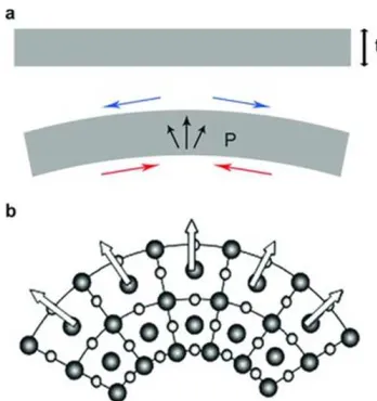
1.1 (a) Flexoelectricity induced by bending. When a slab of thickness tis bent, it results in tension (blue) in one direction and compression (red) in the other, therefore a strain gradient. (b) the zoom-in of the locally bent lat-tices. Center of cations (light color circle) and anions (dark color circle) are displaced. A polarization is induced as a result. From Maranganti et al. (2006). Copyright 2006, American Physical Society. . . 4 1.2 Two most common ways of measuring flexoelectric constants. (a) The
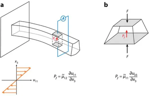
can-tilever beam and (b) the truncated pyramid compression. Gray parts are the electrodes used to measure charge flow. Here, ˜µ12 =µf1122 and ˜µ11 = µf1111.
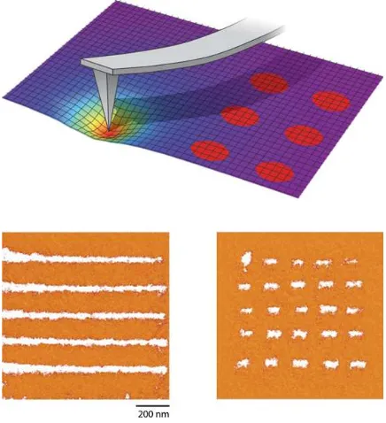
From Zubko et al. (2013). Copyright 2013, Annual Review. . . 5 1.3 Illustration of mechanical writing of ferroelectric polarization by the use of
AFM tip. Strong gradients exerted by the tip can reverse the polarization and hence result in different domain patterns. This method is purely mechanical without any charge injection. From Zubko et al. (2013). Copyright 2013, Annual Review. . . 8
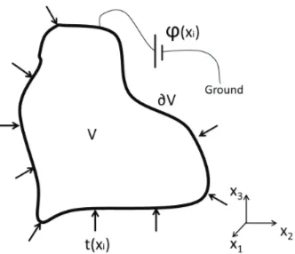
2.1 A deformable dielectric bodyV put in a coordinate system {x1, x2, x3} and
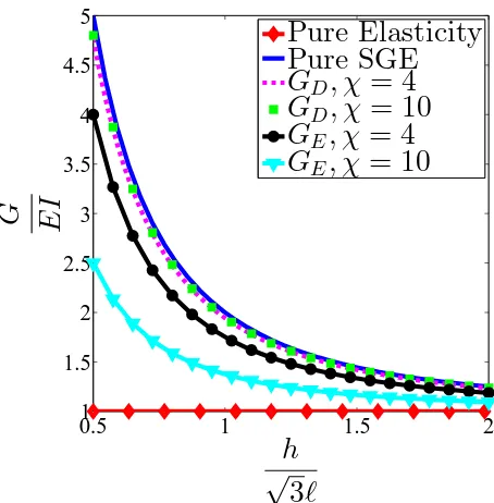
subjected to traction t(xi) and electric loadingφ(xi)on its boundary∂V. . 13 2.2 Size dependent stiffening of flexoelectric beams. Flexoelectric calculations are
carried out keeping ˆfb/fˆm=0.25 where fm=
√
Eℓ2/ǫ
0 and Gis the effective
bending rigidity. . . 23 2.3 A flexoelectric cylindrical tube/disk under pressure and voltage difference. . 25 2.4 This figure plots a) potential and b) polarization with parameters as in
Eqn.(2.71). . . 27 2.5 This figure plots a) radial strain εrr and b) hoop strain εθθ, with parameter
as in Eqn.(2.71). . . 27 2.6 This figure plots a) radial stress σrr and b) hoop stressσθθ, with parameter
as in Eqn.(2.71). . . 28 2.7 This figure plots in (a) the asymptotic behavior of SCF withro/ri→ ∞ and
in (b) the flexoelectric reduction of SCF∞ with increasing ˆf. . . 29 2.8 In this figure, (a) plots SCF∞as a function of potentialV holding mechanical
loads fixed (b) plots polarization at the inner surface as a function of pressure
pi, holding V =0. . . 30 2.9 (a) plots normalized shear strain and (b) the normalized displacement as
3.1 a) plots the comparison of the electric potential induced by a flexoelec-tric defect with f/φ0 = 0.5 and that of a classical point charge with q =
4πǫφf mℓ0exp(−a/ℓ0). b) plots the normalized φf m against the normalized
flexoelectric constants. In here, φ0=
√
(λ+2µ)aǫℓ2/ǫ
0. . . 41
3.2 This figure plots the electric quantities due to an edge dislocation, at θ = π/2. a) plots radial distribution of electric potential with various f’s. b) plots the radial polarization field with different dielectric constants. The curves almost overlap when dielectric constant is larger than 5. Also in here,
φ0=
√
(λ+2µ)aǫℓ2/ǫ
0. . . 45
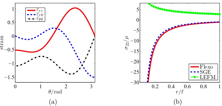
4.1 In this figure, it plots in a) the angular profile of strain at r = ℓ and in b) the σ22 at θ = π/2 for a Mode I & Mode E crack with K4I = 1.0. Material
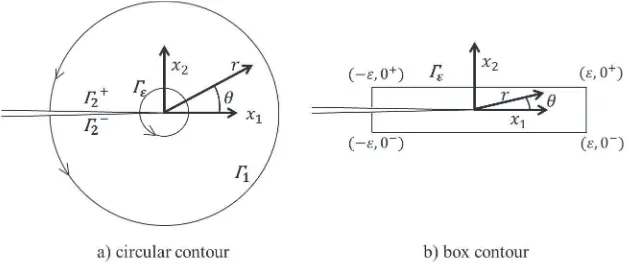
constants are α = 0.5, β = 0.6, ν = 0.3. The intensity factors are from Tsantidis & Aravas (2011) and kept at a constant energy release rate for flexoelectric cases. . . 60 4.2 Contours used in computation of the energy release rate. . . 60 4.3 The COD profile of mixed Mode I & Mode E cracks with different values of
KE. KE is normalized against
√
2πµℓ/ǫ. Other normalized intensity factors are from Tsantidis & Aravas (2011) so as to keep the energy release rate fixed. 64 4.4 This figure plots the electric yielded zone near crack tips for a) Mode I &
Mode E crack, (b) Mode II & Mode D crack. In both cases, ˜DY =1.0 and the crack tip is located atx=0. All material constants are the same as those in Fig.4.1 and Fig.4.3. Notice the similarity of the shape of the electric yielded zone with that of the plastic yielded zone for these cracks. . . 65
5.1 Schematic representation of finite element I9-87. . . 73 5.2 (a) A cylindrical flexoelectric tube with inner and outer radius ri and ro
respectively, is loaded under pressure pi and po, and a voltage difference V across the two surfaces. (b) Finite element mesh used in the calculations (40 elements radially, 20 elements circumferentially). . . 75 5.3 Comparison of finite element and analytical solutions: (a) displacement ur,
and (b) ˜σ(rr2) and ˜σθθ(2), for the tube problem in Fig. 5.2. . . 76 5.4 Radial variation of the electric potential φ (a) and the polarization Pr (b),
for the tube problem in Fig.5.2. . . 77 5.5 (a) A plate with an elliptical hole. (b) Finite element mesh used in the
calculations. . . 78 5.6 Variation of normal strain ε22 (a) and polarization P2 (b) along x1-axis, for
a plate with an elliptical hole as depicted in Fig.5.5 . . . 79 5.7 Contour plots of (a) ε22 and (b) P2 for a plate with an elliptical hole as
de-picted in Fig. 5.5. Loads are prescribed as: σ∞/E=1/200 andω∞/(√a−1E) =
3.2×10⁻³. . . 80 5.8 (a) Mode I insulating crack loaded by uniform distributed load at infinity.
5.10 Predicted polarization field compared to finite element calculation for Mode I insulating crack. (a) is the radial profile and (b) is the angular profile. The closer to the crack tip, the better the calculation agrees with the theory. . . 83 5.11 Predicted rotation Ω3 compared with finite element calculation (Mode D
crack), in (a) radial and (b) angular direction. Note that ω0 is the surface
charge density at bottom. . . 84 5.12 Periodic structure with a repeating unit cell ABCD. . . 85 5.13 Variation of the opening normal strain ε22 (a) and polarizationP2 (b) along
thex1−axis ahead of the void due to a macroscopic strain ¯ε22and an electric
field ¯E2 in the x2−direction, unit-cell under tension . . . 87
5.14 Variation of shear strain ε12 (a) and polarization P1 (b) along the x2− axis
above of the void due to a macroscopic strain ¯ε12 and an electric field ¯E2 in
thex2−direction, unit-cell under shear. . . 88
A.1 In (a), a point load Qis applied, while in (b) there is a potential difference
V between the upper and lower surface over a portion of the beam. . . 95 A.2 Two different arrangements of the bimorph piezoelectric beams with
flexo-electric effects. a) series b) parallel. Beams can be designed to be tail-to-tail (TT) and head-to-head (HH) in terms of poling direction. From Abdollahi & Arias (2015). Copyright 2015, American Society of Mechanical Engineers. 97
Nomenclature
Latin Notations
a Isotropic Reciprocal Susceptibility Constant
a0 Size of a Defect
as Interatomic Spacing
A Cross-section Area
Aijklmn Gradient Elastic Tensor
b Body Force per Volume
bx, bz Components of Burgers Vector
C3, Cij Gradient Elastic Intensity Factors
C Elastic Tensor
Cβ One Edge of ∂V
d Piezoelectric Tensor
D Electric Displacement Vector
Dt Surface Gradient Operator
Dn Normal Gradient Operator
E Electric Field Vector
e Electron Charge
ei Orthonomal Cartesian Basis
E Young’s Modulus
f Flexoelectric coupling tensor
f1, f2 Flexoelectric Coupling Constants
ˆ
fb Effective Bending Flexoelectric Coupling Constant
f Volumetric Flexoelectric Coupling Constant
GD, GE Bending Rigidity
Gij, Gφ Flexoelectric Green’s Function
h Height
H Enthalpy
Ii(⋅), Ki(⋅) ith order Modified Bessel Functions
Jk J Intergral
KE, KD, K4I, II Electric Fracture Intensity Factors
L Geometric Length
ℓℓℓ Unit Outward Normal of an Edge
ℓ Gradient Elastic Length Scale
ℓ1, ℓ2, ℓ0, ℓf Flexoelectric Length Scale
m=n⋅µ˜ Higher-order traction
M Bending Moment
n Unit Outward Normal Vector
pi, po Pressure
pjk=µˆijk,i Divergence of Higher-order Stress
P Electric Polarization Vector
qe Free charge per Volume
qi Coordinates in Reciprocal Space
Q Generalized Traction
Qij Energy Momentum Tensor
r, θ Polar Coordinates
r, θ, z Cylindrical Coordinates
ro, ri Geometric Radius
R Higher-order Traction
s Unit Tangent Vector of an Edge
t Surface Traction
u Displacement Field
uC Displacement on EdgeC
v Shorthand of ui,jnj
V Notation for a General Dielectric Body
∂V Boundary of That Body
V Voltage Difference
w Width
W, WL, WR Energy Storage Density
W(⋅) Work Done by Source (⋅)
AFM Atomic Force Microscopy
BC Boundary Condition
COD Crack Opening Displacement
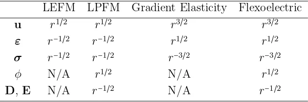
LEFM Linear Elastic Fracture Mechanics
LPFM Linear Piezoelectric Fracture Mechanics
MEMS Micro-Electro-Mechanical System
PFM Piezoresponse Force Microscopy
SCF Stress Concentration Factor
SE Strain Energy
SGE Strain Gradient Elasticity
Greek and Other Symbols
α, β Non-dimensional Flexoelectric Coupling Constants
β Distortion Field
δ Variation
δ0 Defect Mismatch Displacement
δ Identity Tensor
ǫ Dielectric Permittivity Tensor
ǫ0 Permittivity of Vacuum
ǫ Isotropic Dielectric Permittivity
ε Linear Strain Tensor
ε′ Deviatoric Strain
Γ A Closed Contour
κ Curvature of a Beam
λ, µ Lam´e Constants
λe Line Charge Density
ˆ
µ Higher-order Stress in SGE
µf Flexoelectric Tensor
µf1111 Longitudinal Flexoelectric Constant
µf1122 Transverse Flexoelectric Constant
η Concentration Factor
ω Surface Charge Density
Ω Curl of Displacement
Ω Out-of-plane Curl in Plane Problem
ϕ Angle of Twist per Length
σ= (1−ν)/(1−2ν) Non-dimensional Modulus Ratio
σ(0) Cauchy Stress
σ(2)=−∇⋅µ˜ Divergence of Higher-order Stress
σ True Stress Tensor
τ0 Shear Loads
τ Cauchy Stress Tensor
Θ Volumetric Strain or Dilatation
χ Dielectric Susceptibility Tensor
χ Isotropic Susceptibility Constant
∇ Gradient Operator
∂ Partial Differentiation Operator
Li Operator 1−ℓi∇2
∇2 Laplacian Operator
˜
κ Double Displacement Gradient
˜⋅ Type I Formulation
ˆ⋅ SGE or Type II Formulation
¯
(⋅) Average of (⋅)
(⋅)⋆ Fourier Transform of (⋅)
̂
Chapter 1
Introduction
1.1
Flexoelectricity in Hard Materials
Coupled electro-mechanical phenomena are common in nature. For example, strains can be
generated in dielectrics by the application of electric fields through electrostriction. Strains
can also be generated in a special class of dielectrics by the phenomenon of
piezoelectric-ity. Conversely, a piezoelectric material can be polarized when a stress is applied on it.
The study of these phenomena has a long history in mechanics of materials and has been
documented in quite a number of texts, including those of Landau et al. (1984), Maugin &
Eringen (1990), Kovetz (2000) and many others.
A lesser known phenomenon, termed flexoelectricity, is the coupling between
polariza-tion and strain-gradient. Flexoelectricity was first proposed in theory half a century ago by
Mashkevich & Tolpygo (1957), Tolpygo (1963), Kogan (1964) and shortly after, discovered
in experiments by Scott (1968), Bursian et al. (1969). Even though flexoelectricity was first
proposed and found in hard materials, it did not receive much attention within the field of
mechanics of solids largely due to limited means of generating large strain gradients. As
a result, from then on, the study of flexoelectricity has been extensively focused on soft
materials, which can sustain large deformations. Among soft materials, flexoelectricity was
first found to be prominent in liquid crystals Meyer (1969), followed by a systematical
in-vestigation from then on. Readers are referred to the review in Buka & Eber (2012) for
materi-als, like lipid bilayer membranes Raphael et al. (2010), Petrov (2002, 2006), Harland et al.
(2010). It was found that flexoelectricity is related to the mechanism of hearing. Recently
by incorporating fluctuation theory, Liu & Sharma (2013), Deng, Liu & Sharma (2014) also
gave new insights to the subject. But, the origin of flexoelectricity in those materials differ
from hard materials like crystalline solids.
Research on flexoelectricity in hard materials has surged in recent years, largely due
to the advent of modern fabrication and characterization methods. Since gradients scale
inversely as length scales, flexoelectric effects can be greatly enhanced in small specimens.
Flexoelectric polarization also increases as the dielectric constant of a material increases.
Taking account of these scalings, in the last decade high quality specimens of the above
characteristics have been made possible, thanks to the new developments in fabrication
techniques. This has led to a series of experiemental efforts for measuring flexoelectric
constants in different materials. Sophisticated apparatuses for nano-scale characterization,
i.e. atomic force microscopy (AFM), piezoresponse force microscopy (PFM), etc., have
enabled probing this effect at fine scales with high accuracy. In the mean time, significant
growth in computing power stimulates better theoretical approaches to understand the
origins of flexoelectricity. Also, improved numerical and computational tools bring new
perspectives to flexoelectricity and are able to make predictions in more complex contexts.
All these factors contribute to the current revival of interest into flexoelectric phenomena
in hard materials.
1.1.1
Origins of flexoelectricity
Flexoelectricity, by definition, couples electric polarization Pwith strain gradient ∇εin a
linear fashion. Just as a piezoelectric material can be characterized by the piezoelectric
tensord, flexoelectricity can be described by the flexoelectric tensor µf:
Pi=ǫ0χijEj+µfijklεjk,i (1.1)
whereǫ0 is the permittivity of vacuum,χis the dielectric susceptibility tensor andEis the
electric field. In piezoelectricity, d relates electric response (P or electric displacement D)
tensor because strain gradient is a third-order tensor which must be coupled to polarization
vector, a first order tensor.
Early studies of flexoelectricity focused primarily on its microscopic origin. What gives
rise to it? Can we estimate the magnitude of this µf? In what kind of material can we
expect large µf? Kogan (1964) answered these questions by adopting a lattice description
of solids, such as shown in Fig.1.1. Bending of a flat slab introduces a strain gradient along
the cross-section that breaks the local symmetry of the lattice. As a result, the center of
positive and negative charges are displaced, which induces net polarization. In his work, a
straight-forward estimate was calculated by a simple scaling rule:
µf ǫ0χ ≈
e
4πǫ0as ∼
1−10V (1.2)
whereeis the charge of a single electron andasis the interatomic spacing. The above
equa-tion shows that flexoelectricity is directly related to electric susceptibility of the material.
In usual dielectrics, like sodium chloride, whereχ∼10, unless very sharp strain gradient is
created, flexoelectric induced polarization is negligible. This equation also suggests that the
ideal place to observe flexoelectricity is a material with high susceptibility (or high dielectric
constant) that can suffer considerably large strain gradients.
Kogan’s lattice description has long dominated the understanding of flexoelectricity.
In-spired by this, Askar et al. (1970) for the first time numerically calculated the flexoelectric
constants based on shell models. Later, a rigid-ion model was systematically addressed in
Tagantsev (1985, 1991). These works determined the possible contributions to the
flex-oelectric tensor and presented a more rigorous way to compute the ionic contribution to
the relevant constants. Maranganti & Sharma (2009) developed this idea and employed a
lattice dynamic simulation to calculate the flexoelectric constants. However, these works
have been criticized by Resta (2010) since their derivation inevitably involves a surface
contribution. In contrast, Resta (2010) built a more sophisticated physical model which
argued that flexoelectricity, like piezoelectricity, is a purely bulk effect.
Resta’s argument is a first step towards a theory that accounts for both lattice and
electronic contribution to the flexoelectric tensor. In fact, Kalinin & Meunier (2008) for
Figure 1.1: (a) Flexoelectricity induced by bending. When a slab of thickness t is bent, it results in tension (blue) in one direction and compression (red) in the other, therefore a strain gradient. (b) the zoom-in of the locally bent lattices. Center of cations (light color circle) and anions (dark color circle) are displaced. A polarization is induced as a result. From Maranganti et al. (2006). Copyright 2006, American Physical Society.
at a graphene sheet under symmetric bending and found that estimates of the
flexoelec-tric tensor obtained by analytical calculation accounting for the electron clouds around the
carbon atoms are within the range computed by first principles calculation. This was also
the pioneering attempt that used first principles calculation to determine the flexoelectric
tensor. Later, Hong et al. (2010) incorporated this method to study the flexoelectric
prop-erties in BaTiO3, which has been known for its large flexoelectric constants. Subsequent
papers of Hong & Vanderbilt (2011, 2013) systematically derived a complete theory and
first principles simulation framework for general materials, ranging from usual dielectrics
like carbon, diamond and silicon to perovskite ceramics. According to their calculation,
electronic contribution to flexoelectric tensor actually prevails over the ionic contribution in
most of these materials–even in perovskite ceramics for which it was long believed that
flex-oelectricity primarily arises from ionic charge separation. Their results significantly differ
from those of Maranganti & Sharma (2009). Interestingly, although experimentalists often
Figure 1.2: Two most common ways of measuring flexoelectric constants. (a) The cantilever beam and (b) the truncated pyramid compression. Gray parts are the electrodes used to measure charge flow. Here, ˜µ12=µf1122and ˜µ11=µf1111. From Zubko et al. (2013). Copyright
2013, Annual Review.
1.1.2
Quantifying flexoelectric constants
After Kogan (1964), there have been many efforts to measure the flexoelectric constants
µfijkl. As discussed above, an observable flexoelectric effect requires high dielectric constants
and considerably large strain gradients. On the other hand, high dielectric constants can
only be obtained through fabrication of high quality specimens. In the beginning of this
century, Ma & Cross (2001, 2002, 2006) started to look at this problem in some ferroelectric
perovskites in their paraelectric phase. In that phase, not only can we exclude
piezoelec-tricity, but the dielectric constant of these materials can be huge–it can reach as high as
104−105. Ma and Cross managed to measure the transverse flexoelectric constantµf1122 of
these materials using cantilever bending approach, as shown in Fig.1.2(a). Shortly after,
Zubko et al. (2007) used a three point bending system to carry out the measurement on
paraelectric Strontium Titanate. Since bending can only determineµf in part even for
sim-ple cubic materials, as suggested in Zubko et al. (2007), to fully characterize the flexoelectric
tensor, alternative methods must be employed. The truncated pyramid compression method
is one alternative, as shown in Fig.1.2(b). It is employed by Fu et al. (2006), Baskaran et al.
(2011) to measure the longitudinal flexoelectric constant µf1111. Another way of measuring
flexoelectric constants is through Brillouin-scattering, like in Hehlen et al. (1998).
variability in the measurements. For example, the Brillouin scattering method by Hehlen
et al. (1998) inevitably invokes a dynamic flexoelectric effect . The truncated pyramid
compression method is also not reliable. It was intended to set up a uniform strain gradient,
but in reality, as shown in Abdollahi, Mill´an, Peco, Arroyo & Arias (2015), due to the
sharp edges, the strain field inside can be highly inhomogenous. Theoretically, quantifying
flexoelectric constants using beam bending is the most reliable method so far. However,
measurements using this approach also do not converge. Ma & Cross (2001, 2002, 2006)
reported unexpectedly high flexoelectric constants, on the order of 10−100µC/m (exceeding
Kogan’s limit), whereas Zubko et al. (2007) measured it to be on the order of nC/m (within
Kogan’s limit). This discrepancy puzzled researchers for a long time. Not until very recently
was it revealed by Narvaez & Catalan (2014), Garten & Trolier-McKinstry (2015), Narvaez
et al. (2015) that this has to do with other effects due to material properties, such as residual
polarization and flexoelectric poling effect . As observed in M¨uller & Burkard (1979),
Strontium Titanante remains paraelectric at temperature as low as 4K , therefore free of
these concerns. But for other perovskite materials, due to these effects, the flexoelectric
constants measured can be erroneous. Tagantsev & Yurkov (2012) showed that sometimes,
surface effects also perturb the measurement in a non-trivial way. In summary, reliable
methods to determine flexoelectric constants accurately still remain a challenge.
1.1.3
Unique phenomenon due to flexoelectricity
Flexoelectricity, ever since its discovery, has been regarded as an alternative of
piezoelec-tricity at small scales. In fact, as early as the 1960s, Koehler et al. (1962), Turch´anyi, G.
et al. (1973), Whitworth (1975) found that edge dislocations in centrosymmetric materials,
such as sodium chloride, carry charge. Later, Petrenko & Whitworth (1983) extended the
observation to another kind of centrosymmetric material, ice. Piezoelectricity vanishes in
these materials, therefore cannot be the source. Instead, a “pseudo-piezoelectric” effect was
postulated by Evtushenko et al. (1987) for an explanation, which was later shown to be a
result of flexoelectricity Mao & Purohit (2015).
Despite the strong gradient field created by dislocations, it is hardly controllable to
study-response at small scales. Therefore, for piezoelectrics, flexoelectricity can enhance their
piezoresponse. This idea was further demonstrated in simulation studies of Majdoub et al.
(2008a,b) and experimental works of Lee et al. (2011), Qi et al. (2011). At the same time,
Sharma et al. (2007) also predicted that for non-piezoelectrics, piezo-like response can be
manifested through flexoelectric coupling. In fact, Ong & Reed (2012), Duerloo & Reed
(2013) explored this idea using first-principles calculations. They predicted that by
in-troducing non-centrosymmetric defects into 2D symmetric structures, like graphene, an
overall piezoelectric response can be created. Even though introducing atomic size defects
is quite challenging, Zelisko et al. (2014) managed to prove this concept in graphene
ni-tride, experimentally. The response they measured agrees well with predictions made from
flexoelectricity.
However, as noted in Zubko et al. (2013), “flexoelectricity is not just a substitute for
piezoelectricity at the nanoscale; it also enables additional electromechanical functionalities
not available otherwise”. Flexoelectricity opens up the possibility of “gradient
engineer-ing”, an innovative and unique way of optimizing functionalities of electronics. Convincing
evidence of this possibility has already been demonstrated in materials. For instance, it was
discovered that flexoelectricity leads to a gradient induced polarization rotation at a
ferro-electric phase boundary, as shown in Catalan et al. (2011) and that this could lead to a new
mechanism of electronic memory. Lu et al. (2012) further developed this idea by exerting
stress on a BaTiO3 ferroelectric thin film through AFM. In this way, the gradient can be
controlled and flexoelectricity could enable a mechanical way of “writing” polarization into
ferroelectrics as shown in Fig. 1.3. Built upon these results, Oˇcen´aˇsek et al. (2015) explored
the effects of perpendicular point load and sliding loads. Besides, flexoelectric interaction
can also lead to negative domain wall energy as suggested in Borisevich et al. (2012). They
attribute this negative domain wall energy to unusual periodic phase boundaries in an
Sm-doped BiFeO3. Fine structures of ferroelectric domain patterns due to flexoelectricity are
discussed in Ahluwalia et al. (2014).
There has also been some progress in using flexoelectricity at device level. Deng,
Kam-moun, Erturk & Sharma (2014) proposed a flexoelectric energy haverster based on a
can-tilever beam system. Based on a similar idea, a flexoelectric microphone was demonstrated
Figure 1.3: Illustration of mechanical writing of ferroelectric polarization by the use of AFM tip. Strong gradients exerted by the tip can reverse the polarization and hence result in different domain patterns. This method is purely mechanical without any charge injection. From Zubko et al. (2013). Copyright 2013, Annual Review.
and strain relaxation, was utilized for thermal-electric conversion/detection devices as in
Chin et al. (2015). A flexoelectric microelectromechanical system (MEMS) on silicon was
fabricated by Bhaskar et al. (2015) with a performance comparable to the state-of-the-art.
Later, Bhaskar et al. (2016) was able to demonstrate a proof-of-concept strain diode based
on the unique interaction between piezoelectricity and flexoelectricity. Thus, the interest in
novel and unique functionality based on flexoelectricity is increasing.
1.2
Continuum Treatment of Flexoelectricity
The surging interest in flexoelectricity demands a theoretical machinery that predicts
elec-tromechanical response under complex circumstances. The theory of continuum mechanics,
including that of piezoelectricity has been successful in doing so, even in the non-linear
regime. However, since flexoelectricity is a gradient effect, thus size-dependent, it cannot
be directly incorporated into continuum mechanics, which does not possess an intrinsic
strain-gradient elasticity (SGE) or strain-gradient elasticity. The theory of strain-gradient elasticity works well
at small scales (especially sub-micron scales) when non-local phenomenon is prominent.
And we expect the continuum theory of flexoelectricity will work well also within that
range. Gradient elasticity was developed by Mindlin (1964), Toupin (1962), Koiter (1964),
in which strain gradients are included in the elastic strain energy function. Under that
assumption, they have shown that a consistent continuum theory can be derived similar to
the classical one. Later Fleck et al. (1994), Fleck & Hutchinson (1997) extended the theory
to strain-gradient plasticity. Various finite element formulations based on these ideas are
also documented in the literature, e.g., Herrmann (1981), Ramaswamy & Aravas (1998a,b),
Providas & Kattis (2002), Amanatidou & Aravas (2002).
To account for flexoelectricity, the above gradient elasticity framework needs to be
ex-tended to include general electromechanical coupling. Toupin (1956) proposed a variational
principle which later was named after him, for such purposes. This principle was used by
Mindlin (1968) to model other size-dependent electromechanical phenomena.
Flexoelec-tricity can be treated in a similar fashion. Based on this idea, Maranganti et al. (2006)
calculated the Green’s function for flexoelectric solids and used it to examine an Eshelby
problem. Later, Majdoub et al. (2008b) looked at a flexoelectric nanobeam and predicted
a size-dependent flexoelectric stiffening effect. Shen & Hu (2010) provided a general
vari-ational framework for flexoelectric solids including surface effects. Liu (2013) generalized
the framework to large deformations. Besides, Liu & Sharma (2013), Deng, Liu & Sharma
(2014) showed that fluctuation can also be incorporated in the continuum framework. In
the mean time, mesh-free finite element analysis based on continuum models have also
been carried out on more complicated geometries. Abdollahi, Mill´an, Peco, Arroyo & Arias
(2015) revisited the truncated pyramid compression experiments and showed that it is not
reliable by design. Abdollahi et al. (2014), Abdollahi & Arias (2015) gave some new
in-sights and showed how we can further utilize flexoelectric beam structures. Abdollahi, Peco,
Mill´an, Arroyo, Catalan & Arias (2015) looked at the asymmetry of fracture toughness in
flexoelectric materials.
Despite all this theoretical and computational effort into the continuum theories of
flexoelectricity, there has been some inconsitency in the treatment of the SGE terms. In
an intrinsic limit for the magnitude of flexoelectric constants, SGE is also essential to ensure
that the energy storage function is positive definite. Finite element analysis in the presence
of these SGE terms can also be tricky and needs careful treatment as stated in Mao et al.
(2016). However, if these difficulties can be surmounted, many new and useful boundary
value problems can be solved to inspire better application/experimental methods like in Mao
& Purohit (2014), Mao et al. (2016). The interaction between defects and flexoelectricity
can also bring some new insights into this subject as in Mao & Purohit (2015). This
dissertation addresses all the above questions and is based on the aforementioned works
(published or submitted). That said, it is important to point out that flexoelectricity is
a rich subject and there are many other results that are beyond the scope of this thesis.
For those, readers are directed to the following reviews: Nguyen et al. (2013), Zubko et al.
(2013), Yudin & Tagantsev (2013).
1.3
Scope of the thesis
Following the introduction, Chapter 2 gives a systematic way of solving flexoelectric
boundary value problems based on SGE models. First, we deal with general formulation of
flexoelectricity combining SGE and electrostatics. Second, a reciprocal theorem is proved
under linear constitutive law. Third, governing equations of the Navier type are obtained
for isotropic materials. Chapter 2 is then completed by solving a few boundary value
prob-lems (BVP’s) based on this new model. Torsion, beam bending and axisymmetric plane
problems are solved analytically.
Chapter 3 and Chapter 4 extend the framework of Chapter 2 to defects. Defects
create strong discontinuities in a continua and hence large gradients. Flexoelectric
inter-action is expected to be prominent in the neighborhood of defects and die away quickly
in the far field. We analytically quantify this expectation for typical types of defects. In
particular, Chapter 3 deals with point defect and dislocation, where connections to various
experimental results are made. Chapter 4 deals with cracks where unique fracture behaviors
of flexoelectric solids are identified.
Chapter 5 provides a consistent finite element method for flexoelectricity. First, we
with the higher-order differential governing equations due to flexoelectricity. This method
is then implemented and validated against benchmark problems solved in Chapter 2. After
validation, the finite element code is used to study problems involving complicated
geome-tries: elliptical hole in a plate, edge crack panel, and materials with periodic unit cell.
Chapter 6 concludes the dissertation by summarizing and discussing the results of the
Chapter 2
Continuum Theory of
Flexoelectricity
2.1
Introduction
In this chapter, we start our investigation from a general model of flexoelectricity in
con-tinua. In general, as pointed out in Kovetz (2000), Suo et al. (2008), governing equations
of electromechanical phenomena are the Maxwell equations and conservation of linear and
angular momentum. As a special case, electrostatics and linear elasticity combined suffice
as a linear model of piezoelectricity. However, since flexoelectricity has to do with gradient
effects, it has to be modeled with different governing equations and constitutive relations.
As discussed in the introduction, we need to invoke SGE theories to model
flexoelec-tricity. Before doing so we will first review the classical field theory of a dielectric solid
in Section 2.2. We will show the consistency between the classical theory and variational
principles of Toupin (1956). In Section 2.3, we show how Toupin’s variational principles
can be generalized to include general electromechanical coupling. To treat SGE
consis-tently, we follow the treatment of Mindlin (1964), Toupin (1962), Koiter (1964), Fleck et al.
(1994), Fleck & Hutchinson (1997), Aravas (2011). In these theories the energy density
depends both on the strain and its gradient, and an intrinsic material length scale enters
higher order stresses. Some simplified theories, such as Yang et al. (2002), Hadjesfandiari
& Dargush (2011), are also available to deal with special cases where certain components
of the strain gradient can be neglected. In Section 2.4, we further develop the theory
us-ing a general linear constitutive model. A reciprocal theorem is proved. In Section 2.5,
we deal with isotropic flexoelectric materials. Isotropic materials exclude piezoelectricity,
hence isolating flexoelectricity as the source of linear electromechanical coupling. We
de-rive a higher-order Navier Equation. All through this section, SGE is treated consistently.
It is an essential part of flexoelectricity, without which the energy storage function loses
its positive-definiteness. The SGE length scale also provides a bound for the flexoelectric
coupling constants.
Following this general framework, we will use it to solve some one- and two-dimensional
problems that are closely related to experiments. These problems include beam bending,
torsion, cylinders under pressure and shear. We give closed form solutions to each of the
problem. They can be used to interpret experiments on flexoelectric solids and can also
provide a benchmark for verifying continuum based computational methods.
2.2
Classical continuum field theory
Now consider an elastic dielectric body occupying region V with a boundary∂V in
three-dimensional space, as shown in Fig.2.1. Without loss of generality, we will develop our
theory in a Cartesian coordinate system with orthonormal basis{e1,e2,e3} and respective
coordinates {x1, x2, x3}. The body is subject to some mechanical loads. As a response, a
displacement field,u(x)is generated due to deformation. If we constrain ourselves to small
deformations, the linear strain tensor εis sufficient to describe the deformation field of the
body:
εij = 1
2(ui,j+uj,i). (2.1)
This body is dielectric and it has an electric response as well. As pointed out by Suo
et al. (2008), the phenomenon can be intuitively thought of as every material point being
connected to a battery that can pump (or withdraw) charge from it. Therefore, a scalar
Figure 2.1: A deformable dielectric body V put in a coordinate system {x1, x2, x3}
and subjected to traction t(xi)and electric loading φ(xi)on its boundary ∂V.
field is defined as:
Ei=−φ,i, (2.2)
but as we will show shortly after, in more general electromechanical coupling problems, e.g.
those associated with polarization gradient theories, Eqn(2.2) will need some modification.
The deformation and potential fields are the results of loads prescribed on the body.
By the Cauchy postulate, for any continuous tractiont(x)on the surface, there is a second
order tensor σ such that:
σijnj=ti, on ∂V, (2.3)
wherenis the unit outward normal vector of∂V. In classical continuum theory, true stress
and Cauchy stress are equal to each other. But, in couple stress theory or gradient elasticity
theory they are not equal, and we reserve the symbolσ for the true stress. As alluded to
earlier, the battery connected to the material pumps some charge on the surface, with a
density ω, a scalar. Correspondingly, a vector called electric displacement D is uniquely
determined:
Dini=−ω, (2.4)
where a negative sign is kept to obey the convention of electrostatics. These relations keep
the material in equilibrium states and can be generalized to the surface of any control
volume inside the body, therefore, σ and D are well-defined at all the material points.
is due to polarization, the bound charge. These two types of charges summed together give
the “total” charge. Hence,
Di=ǫ0Ei+Pi, (2.5)
whereǫ0 is the permittivity of vacuum. For a linear rigid dielectric, we know
Di =ǫijEj, (2.6)
where ǫ = ǫ0(δ +χ) is what we usually call a dielectric permittivity tensor. χ is the
susceptibility tensor andδ is the identity tensor or Kronecker delta.
All of the above sets up the fundamentals for a continuum field theory of a dielectric
solid. The influence of external sources is reflected by the change of the free energy of the
solid. Suppose the density of the energy storage function is W, then we have:
δW =σijδεij+EiδDi, (2.7)
where δ denotes some small changes or variation in the variable that follows it. Note that
this means we are assumingW =W(ε,D) for the classical continuum theory. According to
Eqn(2.5), we can also work with the polarization, if we remember that
δW =σijδεij+EiδPi+δ(
ǫ0
2EiEi), (2.8)
which is mathematically equivalent. In fact, Toupin’s variational principle is based on this
formulation. To ensure consistency, the energy density he worked with isWL:
WL= W−
ǫ0
2EiEi. (2.9)
Thus, the work conjugate of polarization is the electric field. We can start from a pure
energetic point of view, that is, to assume the work conjugate of ε and P to beσ and E,
respectively, so that
σij =
∂WL
∂εij
, Ei=
∂WL
∂Pi
. (2.10)
theories. In the classical context, we can write Toupin’s variational principle as
∫Vδ(WL− 1
2ǫ0φ,iφ,i+φ,iPi)dV =∫V(biδui−qeδφ)dV+ ∫∂V(tiδui−ωδφ)dS, (2.11)
where, b is the body force per unit volume and qe is the free charge volume density. Note
that this is a general formulation that can deal with the case whereEi≠−φ,i, as in Mindlin
(1968).
Substituting Eqn(2.10) into Eqn(2.11) and analyzing the variational form, we have the
following governing equations:
σij,j+bi=0, (2.12)
Ei+φ,i=0, (2.13)
−ε0φ,ii+Pi,i−qe=0, (2.14)
which recovers the equilibrium equation and the Maxwell equation, and gives the following
boundary conditions:
σijnj−ti=0, on∂Vt, (2.15)
(−ε0φ,i+Pi)ni+ω=0, on ∂Vω, (2.16)
which recovers those of Eqn(2.3, 2.4).
In the following section, we will generalize the above machinery to study flexoelectricity.
2.3
Governing equations
To generalize the above framework to flexoelectricity, the strain gradient εjk,i needs to be
included in the energy density and we define the following pairs of work conjugates:
τij =
∂WˆL
∂εij
, µˆijk=
∂WˆL
∂εjk,i
, Ei=
∂WˆL
∂Pi
, (2.17)
whereτ is the Cauchy stress in the generalized theory and ˆµis the higher-order stress–the
Along with this higher-order stress, there must be a generalized surface load associated
with it, whose conjugate must be related to the gradient of displacement on the surface.
However, once the displacement is given on the boundary, the tangential part of
displace-ment gradient is already determined. Only the normal derivative ∂∂un can be independent
of the displacement on the boundary. Therefore, a higher-order load Rˆ conjugate to ∂∂un
should enter the variational form. As a consequence, the variational form can be written
as:
∫Vδ(WˆL− 1
2ǫ0φ,iφ,i+φ,iPi)dV =∫V(biδui−qeδφ)dV+ ∑β ∮ CTβ
ˆ
Tiuids (2.18)
+ ∫∂V[Qˆiδui+Rˆiδ(ui,jnj)−ωδφ]dS
where ˆQis the generalized traction on ∂V. The boundary integrals on CTβ are included in
Eqn(2.18) when the outer surface ∂V is piecewise smooth; in such a case, the surface ∂V
can be divided into a finite number of smooth surfaces ∂Vβ (β=1,2, . . .) each bounded by
an edge Cβ=Cuβ∪CTβ (Cuβ∩CTβ =∅).
With this we know that the governing equation will be:
τjk,j−µˆijk,ij+bk=0, (2.19)
−ǫ0φ,ii+Pi,i=qe (2.20)
Ei+φ,i=0 (2.21)
In general, there is no free charge in an ideal dielectric, hence qe =0. Equation(2.21) can
be put in a more compact form:
Di,i=0. (2.22)
This equation, along with Eqn(2.19) constitutes the governing equation of a general
di-electric with gradient effects, under small deformations. To model flexodi-electricity, we need
to add constitutive information. These governing equations admit six types of boundary
1. displacement boundary condition
ui=uˆi, on ∂Vu, (2.23)
2. normal derivative boundary condition
Dnui=ˆvi on ∂Vv, (2.24)
3. traction boundary condition
nj(τjk−µˆijk,i)−Dtjniµˆijk−(Dtpnp)ninjµˆijk=Qˆk, on ∂VQ, (2.25)
4. higher-order traction boundary condition
ninjµˆijk=Rˆk on ∂VR, (2.26)
5. potential boundary condition
φ=φˆ on ∂Vφ, (2.27)
6. surface charge boundary condition
niDi=−ωˆ on ∂Vω. (2.28)
There are two additional conditions when∂V has edges :
ui=uˆCi onC β
u, (2.29)
[[ [[
[[ℓjnkµˆkji]]]]]]=Tˆi onCTβ. (2.30)
In all the above boundary conditions, (uˆ,Qˆ,vˆ,Rˆ,uˆC,Tˆ,φ,ˆ ωˆ) are known functions, Dn =
n⋅∇=ni∂x∂i is the normal derivative,Dt=∇−nDnthe “surface gradient” on∂V,∂Vu∪∂VQ=
∂Vv∪∂VR = ∂Vφ∪∂Vω =∂V, and ∂Vu∩∂VQ =∂Vv∩∂VR =∂Vφ∩∂Vω =∅. The double
brackets [[ ]] indicate the jump in the value of the enclosed quantity across Cβ, and an
2.4
Linear constitutive relations
So far, we have given the governing equations for a linear electromechanical theory of
dielectrics with gradient effects. Flexoelectric materials, which are our concern now, are in
the class for which ˆWLis quadratic:
ˆ
WL(εij, εjk,i, Pi)= 1
2Cijklεijεkl+ 1
2Aˆijklmnεjk,iεmn,l+ 1
2aijPiPj, (2.31) +dijkεijPi+fˆijklεjk,iPl,
where C is the fourth order elasticity tensor, ˆA is the strain-gradient elasticity tensor, d
is the piezoelectric tensor, ˆf is the flexoelectric coupling tensor and a is the reciprocal
susceptibility tensor (a=ǫ−01χ− 1
).
According to Eqn(2.17), we obtain the constitutive laws for a flexoelectric material:
τij = Cijklεkl+dijkPk, (2.32)
ˆ
µijk=fˆijklPl+Aˆijklmnεmn,l, (2.33)
El=aljPj+dijlεij+fˆijklεjk,i. (2.34)
Using the governing equations and the linear constitutive relations above, we prove a
re-ciprocal theorem as follows. Consider the solutions to two different problems, the original
problem (problem 1) and the reciprocal problem (problem 2) which we differentiate by
up-per indices 1 and 2. The total work done by the original quantities through their reciprocal
conjugates is
W(12)=
∫V[τij(1)εij(2)+µˆ(ijk1)ε(jk,i2) +Ei(1)Di(2)]dV. (2.35)
W(21), which is the work done by the reciprocal quantities through their original conjugates, can be defined in a similar manner. Applying integration by parts and using the boundary
conditions, we obtain
W(12)=
∫V[−(τjk(1)−µˆ(ijk,i1) ),juk(2)+φ(1)Di,i(2)]dV+∫ ∂V[
ˆ
Plugging in the governing equations Eqn(2.19, 2.22) we get
W(12)=
∫Vb(k1)u(k2)dV+ ∫
∂V[ ˆ
Qi(1)ui(2)+Rˆi(1)v(i2)+φ(1)ω(2)]dS. (2.37)
Thus,W(12)is completely determined by the body force and boundary loads. Alternatively,
W(12) can also be written by use of the constitutive laws:
W(12)=
∫V[Cijklε(kl2)ε(ij1)+aijPi(2)Pj(1)+ǫ0E(i2)Ei(1)+dijk(Pk(2)εij(1)+Pk(1)ε(ij2)) (2.38) +fˆijkl(P(2)
l ε
(1)
jk,i+P
(1)
l ε
(2)
jk,i) +Aˆijklmnε
(2)
mn,lε
(1)
jk,i]dV.
Due to Maxwell relationsC,Aˆ andahave major symmetry, henceW(12) is symmetric with
respect to its upper indices. In other words:
W(12)= W(21). (2.39)
Furthermore, in the absence of body force and higher-order traction, the reciprocal theorem
can be written in a compact form:
∫∂V[Qˆ(i1)ui(2)+φ(1)ω(2)]dS =∫
∂V[ ˆ
Q(i2)u(i1)+φ(2)ω(1)]dS. (2.40)
An example to demonstrate this result is shown in the Appendix A.1.
2.5
Isotropic flexoelectric material
The tensorial nature of the constitutive laws implies a rich variety of flexoelectric materials.
However, in order to understand the general features of a flexoelectric material we must
first study the simplest materials in this class. Therefore, we specialize to an isotropic
flexo-electric material. Isotropic materials cannot be piezoflexo-electric, sod=0. Furthermore, under
only one additional material length scaleℓ, the energy densityWLtakes the following form:
ˆ
WL(εij, εjk,i, Pi)= 1
2λεiiεjj+µεijεij+ 1 2ℓ
2(λε
kk,iεnn,i+2µεjk,iεjk,i) (2.41)
+1
2aPiPj+ (fˆ1εkk,iPi+2 ˆf2εij,iPj),
whereλand µare Lam´e constants and ˆf1and ˆf2 are two flexoelectric coupling constants. a
is the reciprocal susceptibility which is related to the dielectric permittivity ǫ and
suscep-tibility χthrough a−1=ǫ0χ=ǫ−ǫ0. The above isotropic assumption leads to the following
constitutive relations:
τij =λεkkδij+2µεij, (2.42)
ˆ
µijk=(λεpp,iδjk+2µεjk,i)ℓ2+ (fˆ1δjkPi+fˆ2δijPk+fˆ2δikPj), (2.43)
Ei=aPi+fˆ1εkk,i+2 ˆf2εij,j. (2.44)
Substituting the relations above into the governing equations Eqn(2.19, 2.22) and making
use of Eqn(2.1) we get:
∂ii(aǫφ+f uˆ k,k)=0, (2.45)
(λ+µ)(1−ℓ21∂ii)uk,kj+µ(1−ℓ22∂ii)uj,kk=0, (2.46)
where ˆf =fˆ1+2f2 and ℓ1,ℓ2 are some material length scales given by:
ℓ21=ℓ2− ǫ0fˆ 2
(λ+µ)aǫ+
ˆ
f22
(λ+µ)a, ℓ 2 2=ℓ
2−fˆ22
aµ. (2.47)
Note that Eqn(2.46) differs from that of Aravas (2011) in that we have two length scalesℓ1
and ℓ2 while he has only ℓ. We observe from Eqn(2.47) that this is due to the flexoelectric
effect. Interestingly, the form of Eqn(2.46) is the same as the Navier equation of general
strain gradient elasticity proposed by Mindlin & Eshel (1968), but his length scales have
nothing to do with electromechanical coupling. However, Mindlin’s argument concerning
the positive definiteness of the energy still applies here.
Following that argument, in the isotropic flexoelectric material, to ensure
positive-definite (SE is the strain energy). This is because SE is already positive-positive-definite due to the
constrains put on the Lam´e constants:
3λ+2µ>0, µ>0. (2.48)
Since flexoelectricity only has to do with the gradient terms and electric terms, bounds for
them should be derived from WR. Volumetric strain or dilatation Θ and deviatoric strain
ε′ij are defined as:
Θ=εkk, ε′ij=εij− 1
3Θδij. (2.49)
Now, we rewriteWR in terms of these two variables:
WR= 1 2(λ+
2 3µ)ℓ
2Θ,iΘ,i+ (fˆ 1+
2
3fˆ2)Θ,iPi+µℓ
2ε′
ij,jε′ik,k+2 ˆf2ε′ik,kPi+ 1
2aPiPi, (2.50)
where the variation of Θ, ε′ and Pcan all be taken independently. As a result, to ensure
positive definiteness of the above quadratic form, we must have
a(λ+2
3µ)ℓ
2≥ (ˆ f1+
2 3fˆ2)
2
, 1
2aµℓ
2≥ ˆ
f22. (2.51)
Therefore, in general, the thermodynamic constraints for the flexoelectric coupling constants
are
∣fˆ1+2 3fˆ2∣ ≤ℓ
√ (λ+2
3µ)a, ∣fˆ2∣ ≤ℓ
õa
2 . (2.52)
2.6
Application
In this section, several interesting 1D and 2D problems are examined for flexoelectric solids,
including beams, torsion and cylinders under pressure and shear. They are closely related
to experiments and insights are drawn from the closed-form solutions. Two other problems
2.6.1
Euler Bernoulli beam
Consider a slender beam on thee1−e2plane, with length Land thickness 2h(with widthw
ine3 direction). The coordinatex1 runs along the length of the beam through the centroid
of the cross-section and x2 lies along the thickness of the beam. We assume L ≫2h, so
that gradients in the e2 direction are much larger than the gradients in the e1 direction,
e.g. E2≫E1. As an approximation, we only work with the leading order terms here.
Suppose some distributed shear loads q(x1)and a voltage difference V(x1) are applied
on the beam (with lower surface grounded). These loads will contribute to the deflection of
the beam and create a curvatureκ(x1)≈u2,11. From the Euler-Bernoulli theory we have:
ε11=−κx2, ε22=ε33=κνx2, εij =0 otherwise (2.53)
whereν is the Poisson ratio. Under this deformation field, according to Eqn(2.45),
φ= V
2(1+
x2
h )=E2x2+ V
2, (2.54)
where E2 =−V(x1)/2h. Our objective is to determine the curvature κ under given loads.
Given the above strain and potential field, the energy density W can be written in the
following form:
ˆ
W = 1
2(Ex
2
2+Eℓ2−ǫ0χfˆb2)κ2+ 1 2ǫE
2
2 (2.55)
where E is the Young’s modulus and ˆfb = fˆ1−νfˆ is the effective bending flexoelectric
coupling constant. This is the total energy stored in the flexoelectric solid. Based on the
constitutive relations Eqn(2.5) and Eqn(2.44), we also know that
D2=ǫE2+ǫ0χfˆbκ. (2.56)
This equation shows that present day experimental measurements using the beam approach,
e.g. Ma & Cross (2001, 2002, 2006), Zubko et al. (2007) are actually quantifyingµfb =ǫ0χfˆb.
In the above experiments, the beams used for measurements are short-circuited to
mea-sure charge flow. Beams can also be made open-circuited to suffer purely mechanical loads.
energy expressions, viz.
∫V∆ ˆWdV = (ǫ−ǫ0) 2fˆ2
bA
2ǫ ∫
L
0 κ
2dx
1, (2.57)
where A is the cross-sectional area. Open circuit beams have larger energy for the same
amount of deformation. This is the ‘flexoelectric stiffening’ effect which is an enhancement
in the bending rigidity proportional to ˆfb2. This effect is also described in the works of
Majdoub et al. (2008b), Yan & Jiang (2013). A similar effect is also observed in beams made
of piezoelectric materials in Yang (2005) and is known in the literature as ‘piezoelectric
stiffening’. To further elucidate this point, the governing equation for the beam can be
obtained in the following fashion:
M(x1)= ∂ ∂κ∫A
ˆ
W(κ, D2)dS=(EI+EAℓ2−ǫ0χfˆb2A)κ+
ǫ0χfˆbA
2h V. (2.58)
This relation shows that V causes a bending moment as a result of flexoelectric coupling.
Therefore, the governing equation of this beam is
d2M
dx21 =(EI+EAℓ 2−ǫ
0χfˆb2A)
d2κ dx21 +
ǫ0χfˆbA 2h
d2V
dx21 =q(x1). (2.59)
Here, we let GE =EI+EAℓ2−ǫ0χfˆb2A, which is the bending rigidity of the short-circuited
beams. We can also find the bending rigidity of the open circuit beam, GD, in a similar
way and get
GD−GE
EI =
3ǫ20χ2fˆb2
ǫEh2 . (2.60)
Thus, flexoelectric stiffening is related to the flexoelectric coupling constants and the
thick-ness of the material. If the thickthick-ness is small there could be a large flexoelectric stiffening.
This is shown in Fig.2.2.
Beam offer a simple but useful system to study flexoelectricity. There are many other
ways of application, such as in Appendix A.2, where flexoelectricity can be used to alter
0.5 1 1.5 2 1
1.5 2 2.5 3 3.5 4 4.5 5
h
√
3
ℓ
G
E
I
Pure Elasticity
Pure SGE
G
D,
χ
= 4
G
D,
χ
= 10
G
E,
χ
= 4
G
E,
χ
= 10
Figure 2.2: Size dependent stiffening of flexoelectric beams. Flexoelectric calculations are carried out keeping ˆfb/fmˆ = 0.25 where fm = √Eℓ2/ǫ
0 and G is the effective
bending rigidity.
2.6.2
Torsion
Torsion of circular shafts generates a constant strain gradient. Surprisingly, such a strain
gradient does not polarize an isotropic flexoelectric material. To see why, let us start with
the displacement field of a circular shaft under torsion with e3 aligned with the axis of the
shaft:
u1=−ϕx2x3, u2=ϕx1x3, u3=0, (2.61)
whereϕ is the angle of twist per unit length. The strains are:
ε13=−
1
2ϕx2, ε23= 1
2ϕx1. (2.62)
The non-vanishing components of the strain-gradient are ε13,2, ε31,2 and ε23,1, ε32,1. The
flexoelectric coupling energy can then be calculated:
ˆ
no matter which direction polarization takes. As a result a circular shaft made of isotropic
flexoelectric material will not polarize under torsion even though strain gradient effects will
lead to a size dependent torsional rigidity. This result also holds for cubic crystals, in which
the flexoelectric tensor takes the following form:
ˆ
fijkl=fˆ1δjkδil+fˆ2(δijδkl+δikδjl) +fˆ3δijkl, (2.64)
where ˆf3is another flexoelectric constant andδijklis the fourth order Kronecker Delta which
is 1 wheni, j, k, l are all equal and 0 otherwise. If the axis of the shaft is aligned with one
of the sides of the cubic lattice then the flexoelectric coupling energy can be easily shown
to still vanish. Similar results are also observed in screw dislocations in the later section. It
is worthy of mention that for torsion of cross-section other than circular shape, the result
can be very different.
2.6.3
Cylinder under pressure
Next we consider a cylindrical tube under pressure. Calculating the stress in a circular disk
or tube with a central hole under internal and/or external pressure is a classic problem in
linear elasticity, just as calculating the capacitance of a cylindrical capacitor is in
electro-statics. The solution in this simple geometry offers not only a direct comparison to classical
elasticity and SGE, but also some insights into the stress and polarization fields near point
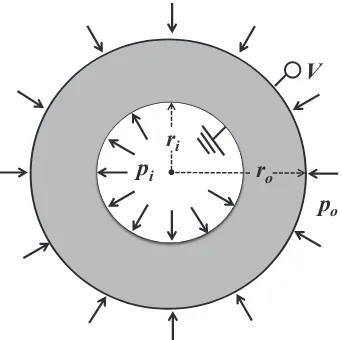
defects in flexoelectric materials. The geometry of the problem is illustrated in figure 2.3.
The cylinder is loaded by internal and external pressures pi and po, and a voltage
difference V is applied across the inner and outer surfaces. The corresponding boundary
conditions are:
ˆ
Qr=−pi, Rˆr=0, φ=0, at r=ri, (2.65)
ˆ
Qr=−po, Rˆr=0, φ=V, at r=ro. (2.66)
It is convenient to solve this axisymmetric problem in polar coordinates so that the only
po ri
ro pi
V
Figure 2.3: A flexoelectric cylindrical tube/disk under pressure and voltage difference.
be simplified to:
(1−ℓ20∇2+ℓ 2 0 r2) (∇
2u
r(r) −
ur(r)
r2 )=0, (2.67)
where∇2 is the Laplacian operator and
ℓ20=ℓ2− ǫ0fˆ 2
a ǫ(λ+2µ), (2.68)
which is the characteristic length scale of this flexoelectric problem. The solution to the
above BVP can be analytically obtained in the following form:
ur(r)=A r+
B
r +C K1( r ℓ0) +
D I1( r ℓ0)
, (2.69)
φ(r)=G+H lnr− fˆ a ǫ(
∂ur
∂r + ur
r ), (2.70)
where(A, B, C, D, G, H) are constants determined from the boundary conditions andIi(x)
andKi(x)theith order modified Bessel functions of the first and second kind respectively.
For detailed component forms of all other quantities, refer to the procedure provided in
Appendix D.
We can solve for these constants, but the expressions are lengthy and uninsightful.