DESIGN AND IMPLEMENTATION OF OPTIMUM INTERPOLATION FILTER USING FARROW STRUCTURE

DESIGN AND IMPLEMENTATION OF

OPTIMUM INTERPOLATION FILTER

USING FARROW STRUCTURE

NAVJOT SINGH

1

University College of Engineering, Punjabi University, Patiala, India1

AMANDEEP SINGH SAPPAL

University College of Engineering, Punjabi University, Patiala, India

Abstract

The Farrow Structure provides an efficient way to implement the interpolation filter using polynomial approximation method for arbitrary sample rate change. The lagrange polynomial approximation method provides almost exact reconstruction of the new interpolated signal as of the input sampled signal. In this paper, cubic lagrange polynomial and 4th order lagrange polynomial approximation methods have been used to implement the design of the interpolation filter based on Farrow Structure. The optimum filter coefficients have been calculated using both polynomial approximation methods. The performance of the two methods has been compared to get the optimum solution to the design of the interpolation filter using Farrow structure.

Key words: Farrow Structure, Interpolation Filter, Lagrange Polynomial Approximation, Multirate Filter.

1. Introduction

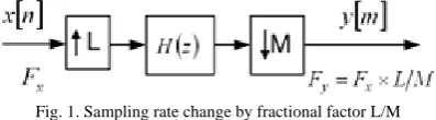
Multirate filters are the digital filters that can increase or decrease the sample rate of the input sampled signal. The examples of multirate filters are the Interpolation and Decimation filters that increases or decreases the sampling rate of a signal respectively. Interpolation is the process of inserting new sample values between existing samples. Interpolation rate change by an integer factor has been used in many modern digital communication systems. This can be easily done using different kind of FIR filters like Equiripple FIR filter, Halfband Filter [1], Root Raised Cosine (RRC) filter or Cascaded Integer Comb (CIC) [10] filter. But in many applications like audio technology, speech coding, echo cancellation in digital modems, symbol synchronisation in digital receivers [3], it is required to interpolate new sample values at arbitrary points between the existing samples. In conventional design, it can be done by first interpolating the signal and then decimating it to obtain an arbitrary fractional rate change using FIR interpolators and decimators in cascade as shown in Fig. 1. The filter

H z

( )

acts as an imaging as well as anti-aliasing filter.

Fig. 1. Sampling rate change by fractional factor L/M

optimum interpolation filter using Farrow structure has been proposed. Section 1 is the introduction; overview of Farrow structure has been discussed in section 2. In section 3, the design and implementation of an optimum interpolation filter using Farrow structure has been presented and section 4 is the conclusion.

2. The Farrow Structure

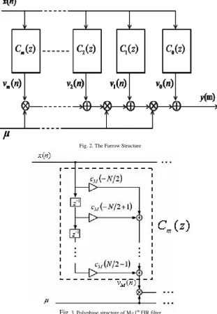
The Farrow structure [2] is an efficient structure to implement polynomial based interpolation filter. Farrow [2] proposed a structure of FIR filters in cascade where the output of each filter is obtained after a delay of a single unit from the previous filter output. The Farrow structure is shown in Fig.2. where

0

( ),

1

( ),

2

( ),...,

M

( )

C z C z C z

C

z

are m+1 FIR filters and each filter has a polyphase structure. Fig. 3. shows the

polyphase structure of a single FIR filter where

c

_M

(

−

N

/ 2),

c

_M

(

−

N

/ 2 1),...,

+

c

_M

( / 2 2),

N

−

c

_M

( / 2 1)

N

−

are the coefficients of polyphase structure of M+1th FIR filter.

v n v n v n

₀

( ), ( ),

_{1 2}

( ),...,

v n

_m

( )

are the outputs of FIR filters respectively. The continuous valued parameter

μ

is called the fractional interval and has values lie between 0 and 1. It controls the fractional factor by which the input sampled signal is to be interpolated and used to determine the time interval between the interpolated output sample and the previous input sample.

Fig. 2. The Farrow Structure

The output signal

y m

( )

of the Farrow structure depends upon the input sampled signal

x n

( )

and response of FIR filters

h t

_c

( )

. Mathematically, the output signal

y m

( )

is given by [10]:

( / 2) 1

/ 2

( )

( )

(

) [(

) ]

N

c l c x

k N

y m

y t

x n k h

k

μ

T

−

=−

=

=



−

+

(1)

Where it is assumed that

n

is the central sample of the interval

−

NT

_x

/ 2

≤ ≤

t

(

NT

_x

/ 2)

−

T

_x and N is an even integer. The impulse response of the Farrow filter is expressed in terms of the coefficients of individual FIR filters and the

μ

factor.

0

[(

) ]

( )

,

M

m

c x m

m

h

k

μ

T

c k

μ

=

+

=



for

k

= −

N

/ 2,

−

N

/ 2 1,...,

+

N

/ 2 1

−

(2)

where

c k c k

₀

( ), ( ),...,

₁

c

M

( )

k

are the coefficients and

M

≤ −

N

1

is the degree of polynomial. When the

polynomial coefficients are known, it is very easy to compute the impulse response for each interval. Now putting Eq. (2) in Eq. (1) we get

( / 2) 1

/ 2 0

( )

(

)

( )

N M

m m

k N m

y m

x n k

c k

μ

−

=− =





=



−



_





_

(3)

or

( / 2) 1

0 / 2

( )

( ) (

)

N M

m

m

m k N

y m

μ

c k x n k

−

= =−





=



−











(4)

or 0

( )

( )

M m m m

y m

v n

μ

=

=



(5)

where

( / 2) 1

/ 2

( )

( ) (

)

N

m m

k N

v n

c k x n k

−

=−

=



−

(6)

( )

m

v n

represents the input/output relationship of the each FIR filter shown in Fig. 2 whose impulse response

coefficients are

c k

m

( )

. Hence transfer function of each FIR filter is given by

( / 2) 1

/ 2

( )

( )

,

N k m m k N

C

z

c k z

−

−

=−

=



where

m

=

0,1,...,

M

(7)

( )

m

C

z

is independent of the value of

μ

and is fixed for a given design. The only variable parameter in the design is

μ

. The output signal

y m

( )

is obtained by adding the multiplication of the outputs of FIR filters by the powers of

μ

respectively.

3. Proposed design of Optimum Interpolation Filter using Farrow Structure

The interpolation filter for any arbitrary interpolation factor can be efficiently implemented using Farrow structure. The design has been implemented in MATLAB using Altera DSP Builder Advanced Blockset. The polynomial approximation methods are used to find the optimum filter coefficients. In most applications, two general classes of polynomials are used: Lagrange Polynomials [7] and B-spline functions [11]. Because the Lagrange approximation method has an advantage of giving the exact reconstruction of the input sample values, hence this method has been used in the proposed Farrow structure based interpolator design. The design has been implemented using 3rd order and 4th order Lagrange polynomials. The polynomial approximation method for 3rd order polynomials is called Cubic Lagrange Interpolation and for 4th order polynomials it is called 4th order Lagrange Interpolation. The coefficients of the polyphase filter stages are computed for cubic lagrange polynomials and 4th order lagrange polynomials. The interpolation factor for the design is set to 1.111 and the input signal is taken as a single frequency sinusoidal signal.

3.1 Implementation using 4th order Lagrange Polynomial

Table 1. Farrow filter coefficients for 4th _{order polynomial}

k m=0 m=1 m=2 m=3 m=4

-2 -0.0018 -0.0090 -0.0198 -0.2536 0.2012 -1 -0.0828 0.0225 0.3287 1.0550 -0.6648

0 0.6587 1.1759 -0.3134 -1.8092 0.9231

1 0.6347 -1.2035 -0.4007 1.5511 -0.6648 2 -0.0827 0.0210 0.3940 -0.5350 0.2012

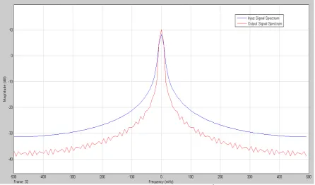
These coefficients are fed to each polyphase partitioned FIR filter. The overall response has been calculated at the output of the interpolation filter. Fig.4. shows the spectrum of the interpolated signal and the input signal for 4th order polynomial coefficients.

Fig. 4. Spectrum of the input signal and the interpolated signal for 4th _{order polynomials}

The response shows that even though the spectrum of the interpolated signal is very much similar to the spectrum of the input signal but the stopband of the interpolated signal has ripples. Hence the response of the interpolation filter does not approximate the ideal filter characteristics.

3.2 Implementation using Cubic Lagrange Polynomial

The filter design for Cubic Lagrange Polynomial consists of four FIR filters which are polyphase partitioned. The filter coefficients for the design are given in Table 2. [10]

Table 2. Farrow filter coefficients for cubic polynomial

k m=0 m=1 m=2 m=3

-2 0 -1/6 0 1/6

-1 0 1 1/2 -1/2

0 1 -1/2 -1 1/2

These coefficients corresponding to each value of

m

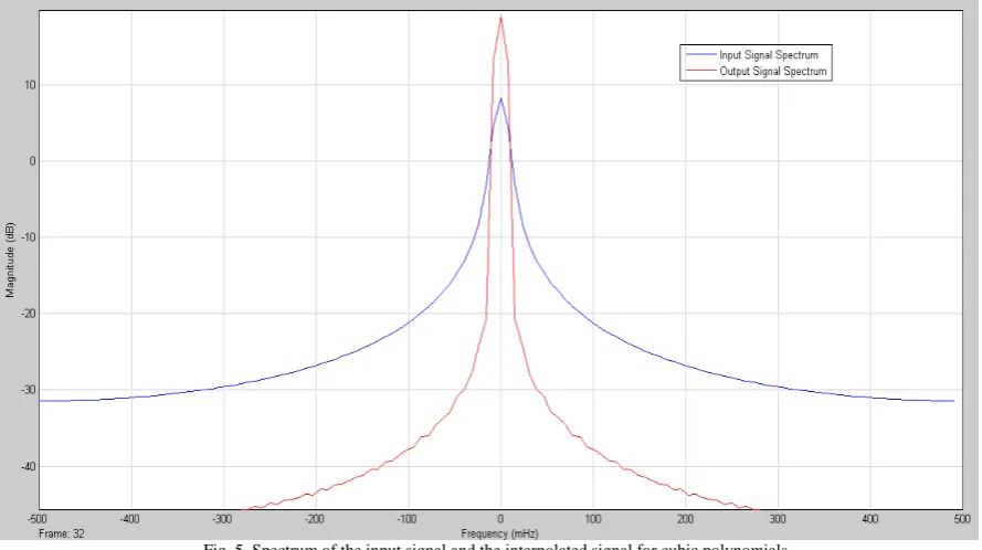
are fed to each polyphase partitioned FIR filter. The overall response has been calculated at the output of the interpolation filter. Fig. 5. shows the spectrum of the interpolated signal and the input signal for cubic polynomial coefficients.

Fig. 5. Spectrum of the input signal and the interpolated signal for cubic polynomials

The response shows that the spectrum of the interpolated signal is very much similar to the spectrum of the input signal. The stopband ripples have been greatly reduced using cubic approximation method. As we know, the higher order polynomials gives more precise reconstruction than the lower order polynomials, but it also increases the ripple content in the interpolation filter output response. Hence, out of the two polynomial approximation methods, the cubic polynomial approximation gives the optimum design of the interpolation filter using Farrow structure because the filter response using this method approximates the ideal filter characteristics.

4. Conclusion

In this paper, the Farrow structure based interpolator design has been implemented using cubic lagrange polynomial approximation method and 4th _{order lagrange polynomial approximation method. The optimal coefficients have been}

obtained for both the polynomial approximation methods. The response of the interpolator using both techniques gives low mean-square error between spectrum of the interpolated signal and the spectrum of the input signal. But the ripple content is more in the interpolated signal of 4th order lagrange polynomial. Hence cubic lagrange approximation method is an optimum method to implement the interplation filter using Farrow structure. The design can be further optimized by using optimal coefficients obtained with some other polynomial approximation methods.

References

[1] R.E. Crochiere and L.R. Rabiner, Interpolation and Decimation of Digital Signals - A Tutorial Review, Proceedings of the IEEE, Vol. 69, No. 3, pp. 300-331, March 1981.

[2] C.W. Farrow, A continuously variable digital delay element, Proc. IEEE Int. Symp. Circuits and Systems, Espoo, Finland, pp. 2641-2645, June 1988.

[3] L. Erup, F.M. Gardner and R.A. Harris, Interpolation in digital modems-Part II: Implementation and Performance, IEEE Trans. Commun., Vol. 41, No. 6, June 1993.

[4] F. Harris, Performance and design considerations of the Farrow filter when used for arbitrary resampling of sampled time series, IEEE transactions, pp. 1745-1749, 1998.

[5] J. Vesma, A frequency domain approach to polynomial based interpolation and the farrow structure, IEEE trans. on Circuits and Systems – II: Analog and Digital Signal Processing, Vol. 47, No. 3, pp. 206-209, March 2000.

[6] J. Vesma and T. Saramaki, Design and properties of Polynomial-based Fractional Delay Filters, IEEE International Symposium on Circuits and Systems, pp. 104-107, May 2000.

[7] A.S.H. Ghadam and M. Renfors, Farrow Structure interpolators based on even order shaped Lagrange polynomials, Proc. of the 3rd International Symposium on image and signal processing and analysis, pp. 745-748, 2003.

[9] Simplifying Simultaneous Multimode RRH design, Altera White Paper, WP-01097, pp. 1-13, March 2009.

[10] L. Milic. Multirate Filtering for digital Signal Processing: MATLAB applications, Information Science Reference, London, United Kingdom, 2009.