State Probability Analysis of Internet Traffic Sharing in Computer Network

---ABSTRACT---

The Internet is a popular electronic tool to access information around the world. It is controlled by large group of network operators and local Internet service providers. The user is a last node of this network. Billions of people around the world are in the club of internet users at present. The growing demand beyond capability is causing congestion and blocking in networks. There is a kind of inherent competition among operators in market to catch-up more and more users. This paper presents Markov chain model based study of state probability in Internet traffic sharing assuming there are only two operators in a local market in competition. Their network blocking probabilities are mutually compared and simulation study is performed over varying model parameters. It is found that some specific type of users are affected much by networks blocking probability.

Keywords - Blocking probability, Call-by-call basis, Initial preference, Internet Service Provider [operators], Internet access, Internet traffic, Morkov chain model, Network congestion, Quality of service (QoS), Simulation, Transition probability, Transition probability matrix, Users behavior .

--- Paper submitted: 10 Jun 2009 Accepted: 13 Sep 2009

---

I. INTRODUCTION

he facility of Internet is spread out over the world and a large number of people are using this for communication media for their purpose. This fact is leading to a high amount of traffic load on the network due to rigorous generation of calls per second. Additional traffic load constitutes to cause congestion in the flow of information in network. In order to improve their customer base, many operators offer marketing packages to attract on their users. Consumers also desire to have better quality of service from providers. Some users are dedicated to their favourate operators only whereas others are occasion-oriented. Naldi (2002) has discussed a Markov chain model based approach to analyze user’s behavior in set up of two operator’s environment. This paper provides an extension of this with the addition of one more state in the model. The additional state is an attraction towards the users comfort. Some useful contribution over model based study are due to Naldi (1999) with theories, techniques of Medhi (1991), Perzen (1962),

Yuan and Lygeros (2005), Shukla et al.(2007,2009), Shukla and Jain(2007).

II. USER'S BEHAVIOR AND MARKOV CHAIN MODEL Let ISP1 and ISP2 are two Internet service providers in a

market. Further, Assume the following for behavior of a user during Internet access:

(i) A user connects his call through either ISP1 or by ISP2.

(ii) The user attempts for an ISP, only once and then shift to the next ISP in next attempt and so on. This behavior is termed as call-by-call.

(iii) There are three other options for a user like (a) go for rest (b) abandon the process (c) get success during call connection. The (a) adopts some new marketing plans with probability PR.

(iv) The initial probability of selection for ISP1 is p, and for

ISP2 is (1-p).

(v) The blocking probability experienced by the operator ISP1 is L1 and by ISP2 is L2.

State Probability Analysis of Internet Traffic

Sharing in Computer Network

Diwakar Shukla

Department of Mathematics and Statistics, Sagar University, Sagar M.P. 470003, India.

Email: [email protected] Sanjay Thakur

Department of Computer Science & Applications, Sagar University, Sagar M.P. 470003, India.

Email: [email protected] Arvind Kumar Deshmukh

Department of Computer Science & Applications, Sagar University, Sagar M.P. 470003, India.

Email: [email protected]

Let {Y(n) _{, n ≥ 0}be a Markov chain having transitions}

over the state space {ISP1, ISP2, RS, SS, AP}, where Y(n)

denotes the position of Y at the nth _{attempts (n ≥ 0), and five}

states are

State ISP1 : first Internet service provider. State ISP2 : second Internet service provider. State RS : taking rest for a short duration State SS : success obtained in call connection State AP : leaving the process for call attempt Suppose the user is on ISP1 in the nth attempt. If this call

blocks with the probability L1 then he may choose either

to ISP2 or to RS state in (n + 1)th attempt. User can not be

at the same state in two successive call attempts except SS and AP. He can abandon the attempt process at (n + 1)th

attempt with probability PA. If reaches to RS from ISP2 in

nth _{attempts then in (n + 1)}th _{attempt he may either with a call}

on ISP1 with probability r or on ISP2 with probability (1 - r).

From RS, user can not move to states SS and AP. The diagrammatic form of transition mechanism in the setup of two Internet service providers is given in fig. 1

SS

AP

ISP₂

ISP1

L1

L2

1-L₂ 1-L₁

1

L₁ P_{A L}

2 PA

1

r 1-r

L1(1-PA) PR L2(1-PA) PR RS

Fig 1 (Transition diagram)

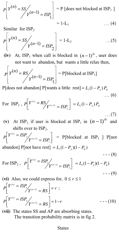
III. TRANSITION PROBABILITIES

(i) The initial probabilities are P Y =ISP =p

  



1 ) 0

( _{; (1 )}

2 ) 0 (

p ISP

Y

P = = −

  



- - - (1) (ii) If

(

n

−

1

)

th attempt call for ISP1 is blocked, the user

may abandon the process in next attempt.

  

 ₌ − ₌

1 ) 1 ( )

(

ISP n

Y AP n Y

P

A P L

1

= - - - (2)

Similar for ISP2,

  

 

  

 

= − =

2 ) 1 ( ) (

ISP n

Y AP n Y

P = L2 PA

- - - (3) (iii) At ISP1 the

n

th attempt call may be made successful

and user reaches to SS from ISP1.

  

 

  

 

= − =

1 ) 1 ( ) (

ISP n

Y SS n Y

P = P [does not blocked at ISP1 ]

= 1-L1 - - - (4)

Similar for ISP2

    

    

= − =

2 ) 1 ( ) (

ISP n

Y SS n Y

P = 1-L2 - - -(5)

(iv)

At, ISP1 when call is blocked in (n−1)th, user does

not want to abandon, but wants a little relax then,

    

    

= − =

1 ) 1 ( ) (

ISP n

Y RS n Y

P = P[blocked at ISP1]

P[does not abandon] P[wants a little rest]=L1(1−PA)PR - - - (6)

For ISP2 , _ = − _{= }

2 ) 1 ( ) (

ISP Y

RS Y

P n

n

R A P P L₂(1− )

=

- - - (7) (v) At ISP1, if user is blocked at ISP1 in

(

n

−

1

)

th and

shifts over to ISP2.   



= =

−

1 ) 1 ( 2 ) (

ISP Y

ISP Y

P n

n

= P[blocked at ISP1 ] P[not

abandon] P[not have rest] =L1(1−PA)(1−PR)

- - - (8) For ISP2 ,

  



= =

−

2 ) 1 ( 1 ) (

ISP Y

ISP Y

P n

n

) 1 )( 1 (

2 PA PR

L − −

=

- - - (9)

(vi) Also, we could express for, 0≤r≤1

r RS Y ISP Y

P n

n

=

  



= =

−1) ( 1 ) (

;

r RS Y ISP Y

P n

n

− =

  



= =

−1) 1

( 2 ) (

- - - (10)

(vii) The states SS and AP are absorbing states. The transition probability matrix is in fig 2.

States (n)

Y

ISP1 ISP2 RS SS AP ISP1

0

L1(1−PA)(1−PR) L1(1−PA)PR 1−L1 L1PA ISP2 L2(1−PA)(1−PR)

0

L2(1−PA)PR 1−L2 L2PA

) 1 (n−

Y RS r 1−r 0

0

0

SS

0

0

0

1

0

AP

0

0

0

0

1

IV. QUALITY OF SERVICE (QOS)

The quality of service (QoS) provided by an ISP is a function of blocking probabilities (L1 and L2) faced by

internet service providers due to congestion in the network. Higher level of blocking probability leads to lesser quality received by users. As per assumptions of the system, a user is suppose to attempt for calls between ISP1 and ISP2 until

connects or may take rest if fed-up due to attempt process.

V. USER’S CATEGORIZATION

Based on position of system in n attempts, one gets: (a) Faithful User (FU):

Who is faithful to ISP1 otherwise prefer for the rest

state RS or abandon but does not attempt for ISP2. The

converse of same is for ISP2. A group of this kind is defined

as faithful users for ISP1 {or ISP2.}. (b) Partially Impatient User (PIU):

Who attempts only between the two service providers ISP1 and ISP2, all the time until call completes or abandon

but never goes to RS.

(c) Completely Impatient User (CIU):

User who attempts to ISP2 or goes to rest state RS in

the _(n+1)th _{attempt when was at ISP}

1 in the nth. Moreover,

when was at ISP2, moves to either ISP1 or on RS in the next. THEOREM 1: The nth step transitions probability for FU to ISP1 is

PY n =ISP =pEn     1 ) 2

( _{; 0}

1 ) 1 2 ( + _{= =}   

 n _ISP

Y

P

where B1=L1(1−PA)PR,E=B1r and n = 0,1,2,3 -PROOF: At n=0, _{P Y =ISP =p}

    1 ) 0

( _{and since, the}

transition over ISP2 from ISP1 is restricted, therefore

following (11), the start of attempt is restricted to ISP1

onlyP_Y(0)=RS_=0

[

] [

]

1 (0) 0

) 1 ( ) 0 ( 1 ) 1 ( ₌     = = = =

=ISP PY RS P Y ISP_{Y RS}

Y P

[

] [

]

1

1 ) 0 ( ) 1 ( 1 ) 0 ( ) 1 ( pB ISP Y RS Y P ISP Y P RS Y P =     = = = = =

[

] [

]

pBr

RS Y ISP Y P RS Y P ISP Y

P 1 (1) 1

) 2 ( ) 1 ( 1 ) 2 ( ₌     = = = = =

[

] [

]

0

1 ) 1 ( ) 2 ( 1 ) 1 ( ) 2 ( ₌     = = = =

=_{RS PY ISP P} Y RS_{Y ISP}

Y P

[

] [

]

1 (2) 0

) 3 ( ) 2 ( 1 ) 3 ( ₌     = = = =

=ISP P Y RS P Y ISP_{Y RS}

Y P

[

] [

]

pB r

ISP Y RS Y P ISP Y P RS Y

P ₁2

1 ) 2 ( ) 3 ( 1 ) 2 ( ) 3 ( ₌     = = = = =

[

] [

]

2 2

1 ) 3 ( 1 ) 4 ( ) 3 ( 1 ) 4 ( r pB RS Y ISP Y P RS Y P ISP Y P =     = = = = =

[

]

[

]

0

1 ) 3 ( ) 4 ( 1 ) 3 ( ) 4 ( ₌     = = = =

=_{RS P Y ISP P} Y RS_{Y ISP}

Y

P

[

] [

]

1 (4) 0

) 5 ( ) 4 ( 1 ) 5 ( ₌     = = = =

=ISP PY RS P Y ISP_{Y RS}

Y P

[

] [

]

3 2

1 1 ) 4 ( ) 5 ( 1 ) 4 ( ) 5 ( r pB ISP Y RS Y P ISP Y P RS Y P =     = = = = =

On continuing in similar way, the proof of the theorem exits.

THEOREM 2: The

n

th step transitions probability for FU to ISP2 isPY(2n)=ISP₂ =(1−p)Dn

  

 _;

P_Y(2n+1)=ISP_2=0 where B2 =L2(1−PA)PR, D=B2(1−r)

THEOREM 3: For PIU the nth step transition probability is:- n pC ISP n Y

P = =

    1 ) 2 ( _; n C A p ISP n Y

P_ (2 +1)= _1=(1− ) ₂

n C p ISP n Y

P (2 )= ₂ =(1− )     _; n C pA ISP n Y

P (2 +1)= ₂ = ₁

  



where A1 = L1(1-PA) (1-PR), A2 = L2(1-PA) (1-PR), C = A1 A2 THEOREM 4: For CIU, the

n

th attempt approximate expressions are, n E C p ISP n Y

P (2 )= ₁ = ( + )

    _; n E D C A p ISP n Y

P (2 +1)= ₁ =(1− ) ₂( + + )

    n D C p ISP n Y

P_ (2 )= _2=(1− )( + ) ; n E D C pA ISP n Y

P_ (2 +1)= ₂_= ₁( + + )

VI. SIMULATION BASED STATE PROBABILITY ANALYSIS The expressions obtained in the theorem 1- 4 are examined through a graphical pattern for increasing number of attempts (n). Fig. 3 reflects that transition probability of ISP1 varying over blocking probability L1 and n. When L1

increases, the chances of transition from ISP1 also increases

but the amount of this variation is very small. For example, at n = 2, we get

  

 ₌

1 2) _ISP (

Y

P = 0.124, when L1 = 0.3,

  

 ₌

1 2) _ISP (

Y

P = 0.204, when L1 = 0.5

and     ₌ 1 2 ISP ) ( Y

P = 0.364, when L1 = 0.8.

While comparing ISP1 with ISP2 over n = 2, 

 

_Y(2) _=ISP1

P = 0.124, when L1 = 0.5 and

  

_Y(2)_=ISP2

P = 0.164, when L2 = 0.5, one can find that

with p = 0.8 for ISP1, at n = 2 ISP2 has better chance than

With the increasing number of attempts the term 0

1 = =

  

 (n) _ISP

Y

P as n→∞. This is interesting to

observe that transition probabilities

  

 ₌

1

ISP ) n ( Y

P is zero

in odd attempts (when n < 8). Fig. 4 is very similar to fig. 3

and supports the fact that the transition

  

 ₌

2

ISP ) n ( Y P

varies over increasing blocking probability for even attempts. This also constantly reduces over large n.

0. 004 0. 044 0. 084 0. 124 0. 164 0. 204 0. 244 0. 284 0. 324 0. 364 0. 404 0. 444 0. 484 0. 524 0. 564 0. 604 0. 644 0. 684 0. 724 0. 764

0 1 2 3 4 5 6 7 8

N o. of a ttempts (n)

S

tat

e p

ro

b

a

b

il

it

y (

P

[Y

(n

)=IS P1

])

L1=0.3 L1= 0.5 L1=0 .8

0. 004 0. 044 0. 084 0. 124 0. 164 0. 204 0. 244 0. 284 0. 324 0. 364 0. 404 0. 444 0. 484 0. 524 0. 564 0. 604 0. 644 0. 684 0. 724 0. 764

0 1 2 3 4 5 6 7 8

No. of attempts (n)

S

ta

te

pr

ob

ab

il

it

y

(

P

[Y

(n

)=I

S

P

2

])

L2=0.3 L2=0.5 L2=0.8

0.004 0.06 0.116 0.172 0.228 0.284 0.34 0.396 0.452 0.508 0.564 0.62 0.676 0.732 0.788

0 1 2 3 4 5 6 7 8

S

ta

te

p

ro

b

a

b

ilit

y

(

P

[Y

(n

)=IS P1

])

L1= 0.3 L1= 0.5 L1= 0.8

0.0040.03 0.056 0.082 0.108 0.1340.16 0.186 0.212 0.238 0.2640.29 0.316 0.342 0.368 0.3940.42 0.446 0.472 0.498 0.5240.55 0.576

0 1 2 3 4 5 6 7 8

S

ta

te

p

ro

b

a

b

ilit

y

(

P

[Y

(

n)=I

S

P2

])

L1=0.3 L1=0.5 L1=0.8

0.0040. 05 0.096 0.142 0.188 0.2340. 28 0.326 0.372 0.418 0.4640. 51 0.556 0.602 0.648 0.6940. 74 0.786

0 1 2 3 4 5 6 7 8

S

tat

e

p

ro

b

ab

il

it

y

(P

[Y

(n

)=I

S

P1

])

L1=0.3 L1=0.5 L1=0.8

0.0040.03 0.056 0.082 0.108 0.1340.16 0.186 0.212 0.238 0.2640.29 0.316 0.342 0.368 0.3940.42 0.446 0.472 0.498 0.524 0.55 0.576

0 1 2 3 4 5 6 7 8

S

tat

e p

ro

b

ab

ili

ty

(P

[Y

(n)=

IS

P2

])

L1= 0.3 L1= 0.5 L1= 0.8

0.0040.05 0.096 0.142 0.188 0.2340.28 0.326 0.372 0.418 0.4640.51 0.556 0.602 0.648 0.6940.74 0.786

0 1 2 3 4 5 6 7 8

S

ta

te

p

r

o

b

a

b

ilit

y

(

P

[

Y

(n

)=I

S

P1

]

)

L1=0.3 L1=0. 5 L1=0.8

0.00 4 0 .0 3 0.05 6 0.08 2 0.10 8 0.13 40 .1 6 0.18 6 0.21 2 0.23 8 0.26 4 0 .2 9 0.31 6 0.34 2 0.36 8 0.39 4 0 .4 2 0.44 6 0.47 2 0.49 8 0.52 4 0 .5 5 0.57 6

0 1 2 3 4 5 6 7 8

S

tat

e p

ro

b

ab

ili

ty

(

P

[Y

(n

)=I

S

P2

])

L1=0.3 L1=0. 5 L1=0. 8

Fig. 3 For FU of operator ISP1

(PA = 0.02, p = 0.8, PR = 0.8, r = 0.03 )

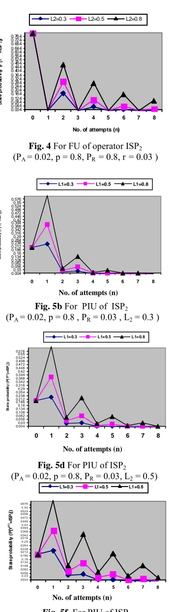
Fig. 4 For FU of operator ISP2

(PA = 0.02, p = 0.8, PR = 0.8, r = 0.03 )

Fig. 5a For PIU of ISP1

(PA = 0.02 , p = 0.8 , PR = 0.03 , L2 = 0.3 )

No. of attempts (n) _{No. of attempts (n)}

Fig. 5b For PIU of ISP2

(PA = 0.02, p = 0.8 , PR = 0.03 , L2 = 0.3 )

No. of attempts (n) No. of attempts (n)

Fig. 5c For PIU of ISP1

(PA = 0.02, p = 0.8, PR = 0.03, L2 = 0.5)

Fig. 5d For PIU of ISP2

(PA = 0.02, p = 0.8, PR = 0.03, L2 = 0.5)

No. of attempts (n) No. of attempts (n)

Fig. 5e For PIU of ISP1

(PA = 0.02, p = 0.8, PR = 0.03, L2 = 0.8)

Fig. 5f For PIU of ISP2

0. 004 0.06 0. 116 0. 172 0. 228 0. 284 0.34 0. 396 0. 452 0. 508 0. 564 0.62 0. 676 0. 732 0. 788

0 1 2 3 4 5 6 7 8

S

ta

te p

r

o

b

ab

il

it

y

(

P

[

Y

(n)=

IS

P1

]

)

L1=0.3 L1=0.5 L1=0.8

0. 0040.03 0. 056 0. 082 0. 108 0. 1340.16 0. 186 0. 212 0. 238 0. 2640.29 0. 316 0. 342 0. 368 0. 3940.42 0. 446 0. 472 0. 498 0. 5240.55 0. 576

0 1 2 3 4 5 6 7 8

S

tat

e

p

ro

bab

ili

ty

(

P

[Y

(n

)=I

S

P

2

])

L1=0.3 L 1= 0. 5 L1=0. 8

0.0040.05 0.096 0.142 0.188 0.2340.28 0.326 0.372 0.418 0.4640.51 0.556 0.602 0.648 0.694 0.74 0.786

0 1 2 3 4 5 6 7 8

S

ta

te

pr

oba

bi

li

ty

(

P

[Y

(n

)=IS

P

1

])

L1=0.3 L1=0.5 L1=0.8

0.0040.03 0.056 0.082 0.108 0.1340.16 0.186 0.212 0.238 0.2640.29 0.316 0.342 0.368 0.3940.42 0.446 0.472 0.498 0.5240.55 0.576

0 1 2 3 4 5 6 7 8

Sta

te

proba

b

il

ity

(P[Y

(n

)=IS

P

2

])

L1=0.3 L1=0.5 L1=0.8

0.0040.05 0.096 0.142 0.188 0.2340.28 0.326 0.372 0.418 0.464 0.51 0.556 0.602 0.648 0.6940.74 0.786

0 1 2 3 4 5 6 7 8

S

ta

te

pr

oba

bi

li

ty

(

P

[Y

(n

)=I

S

P

1

])

L1=0.3 L1=0.5 L1=0.8

0.004 0.03 0.056 0.082 0.108 0.1340.16 0.186 0.212 0.238 0.264 0.29 0.316 0.342 0.368 0.394 0.42 0.446 0.472 0.498 0.5240.55 0.576

0 1 2 3 4 5 6 7 8

S

ta

t

e

p

r

o

b

a

b

ilit

y

(

P

[Y

(n

)=IS P2

])

L1=0. 3 L1=0.5 L1=0.8

According to fig. 5a, 5c, 5e, the competitor's blocking probability affects the PIU state probability because when L1

and L2 both are high; chances to ISP1 are also high. From

fig. 5b, 5d and 5f, one can find that for large number of attempts, the transition probability reaches to zero with the joint condition of large L1 and L2. At n = 1, the highest

transition probability found, followed by next highest at n = 3 for ISP2, but this highest amount decreases with

increasing L2.

In another comparison, when n = 2 and n = 4, L1, L2, kept

fixed, we have

  

_Y(2)_=ISP1

P = 0.142, when L1 = 0.5, L2 = 0.5,

  

 ₌

2 ) 2

( _ISP

Y

P = 0.212, when L1 = 0.5, L2 = 0.5

    

 

 ₌

1 ) 4 (

ISP Y

P = 0.004, when L1 = 0.5, L2 = 0.5

    

 

 ₌

2 ) 4 (

ISP Y

P = 0.056, when L1 = 0.5, L2 = 0.5.

In second attempt, the chance for ISP2 are high and

continues for fourth attempt also, but this difference reduces over increasing n. PIU prefers to ISP2 more up to fourth

attempt even when p = 0.8 for ISP1 exists. This is PIU

behavior. No. of attempts (n)

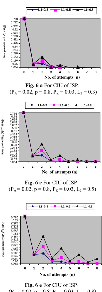
Fig. 6 a For CIU of ISP1

(PA = 0.02, p = 0.8, PR = 0.03, L2 = 0.3)

No. of attempts (n)

Fig. 6 b For CIU of ISP2

(PA = 0.02, p = 0.8, PR = 0.03, L2 = 0.3)

Fig. 6 c For CIU of ISP1

(PA = 0.02, p = 0.8, PR = 0.03, L2 = 0.5)

No. of attempts (n) _{No. of attempts (n)}

Fig. 6 d For CIU of ISP2

(PA = 0.02, p = 0.8, PR = 0.03, L2 = 0.5)

No. of attempts (n)

Fig. 6 e For CIU of ISP1

(PA = 0.02, p = 0.8, PR = 0.03, L2 = 0.8)

Fig. 6 f For CIU of ISP2

In light of fig. 6a, 6c, and 6e, the same pattern found as discussed for PIU. The increase in L2 constantly produces

significant increase in transitions for increasing L1. Similar

happens in fig. 6b, 6d and 6f. For small opponent’s blocking leads to less number of attempts in order to reach the transition probability equal to zero. More and more attempts are needed to stabilize the transition process if L1 and L2

both are towards higher side. So, behavior of CIU are same as PIU in terms of state probabilities.

I. CONCLUDING REMARKS

State probabilities depend on number of call attempts made by user for getting Internet connected. This probability reduces sharply as attempt increases. The FU users have a tendency to stick with their favourate operators up to seven to eight attempts but PIU group has negative tendency in this regards. In contrary, CIU users bear a better proportion of state probabilities. When blocking of the network of ISP1 is

high then he gains state probabilities related to FU users. Moreover, the increase of L2 provides gain in terms of

higher proportion of traffic of ISP1.

REFERENCES

[1] Medhi, J. Stochastic Processes, Wiley Eastern Limited (Fourth reprint), New Delhi, 1991.

[2] Naldi, M. “Internet Access Traffic Sharing in a Multi-user Environment”, Computer Networks, vol. 38, pages 809-824, 2002.

[3] Naldi, M., “Measurement Based Modeling of Internet Dial-up Access Connections”, Computer Networks, 31(22) pages 2381-2390, 1999.

[4] Perzen, Emanual, Stochastic Processes, Holden -Day, Inc., San Francisco, and California,1992

[5] Shukla, D., Gadewar, S., “Stochastic model for cell movement in a Knockout Switch in computer networks”, Journal of High Speed Network, vol. 16, no.3, pp. 310-332, 2007.

[6] Shukla, D., Gadewar, S., Pathak, R., K., “A stochastic model for Space-Division Switches in computer networks”, Applied Mathematics and Computation (Elsevier Journal), vol. 184, Issue 2, pp. 235-269, 2007.

[7] Shukla, D. and Jain, Saurabh. “A Markov chain model for multi-level queue scheduler in operating system, Proceedings of the International Conference on Mathematics and Computer Science, ICMCS-07, pp. 522-526., 2007.

[8] Shukla, D., Tiwari, M., Thakur, Sanjay, Tiwari, Virendra, “Rest State Analysis of Internet Traffic Distribution in multi-operators environment”, Journal of Management and Information Technology (JMIT), vol. 1, pp. 72-82, 2009.

[9] Yeian, C. and Lygeros, J., “Stabilization of a Class of Stochastic Differential Equations with Markovian Switching” System and Control Letters, 9, pages 819-833, 2005.

Author’s Biography

Dr. Diwakar Shukla is working as an Associate Professor in the Department of Mathematics and Statistics, Sagar University, Sagar, M.P. and having over 20 years experience of teaching to U.G. and P.G. classes. He obtained M.Sc.(Stat.), Ph.D.(Stat.), degree from Banaras Hindu University, Varanasi and served the Devi Ahilya University, Indore, M.P. as a Lecturer over nine years and obtained the degree of M. Tech. (Computer Science) from there. During Ph.D., he was junior and senior research fellow of CSIR, New Delhi qualifying through Fellowship Examination (NET) of 1983. Till now, he has published more than 55 research papers in national and international journals and participated in more than 35 seminars / conferences at national level. He is the recipient of MPCOST Young Scientist Award, ISAS Young Scientist Medal, UGC Career Award and UGC visiting fellow to Amerawati University, Maharashtra. He also worked as a selected Professor to the Lucknow University, Lucknow, U.P., for one year and visited abroad to Sydney (Australia) and Shanghai (China) for conference participation. He has supervised seven Ph.D. theses in Statistics and Computer Science both; and eight students are presently enrolled for their doctoral degree under his supervision. He is member of 10 learned bodies of Statistics and Computer Science both at national level. The area of research he works for are Sampling Theory, Graph Theory, Stochastic Modelling, Computer Network and Operating Systems.

Dr. Sanjay Thakur has completed M.C.A. and Ph.D. (CS) degree from H.S. Gour University, Sagar in 2002 and 2009 respectively. He is presently working as a Lecturer in the Department of Computer Science & Applications in the same University since 2007. He did his doctoral work in the field of Computer Networking and Internet traffic sharing. He has authored and co-authored 10 research papers in National/International journals and conference proceedings. His current research interest is Stochastic Modeling of Switching System of Computer Network and Internet Traffic Sharing Analysis.