A Novel Color Face Recognition with Semi-orthogonal MPCA Method

(1)

Krissada Asavaskulkiet

*

Department of Electrical Engineering, Mahidol University, Nakorn Pathom, Thailand.

* Corresponding author. Email: [email protected] Manuscript submitted January 10, 2019; accepted March 8, 2019. doi: 10.17706/ijcce.2019.8.2.73-82

Abstract: In this paper, the semi-orthogonal multi-linear principal component analysis (MPCA) method has been proposed for color face recognition. Recently, MPCA seems to be an appropriate scheme for dimensionality reduction and feature extraction from color images, handling the color channels in a natural, “holistic" manner. However, it is difficult to develop an effective MPCA method with the orthogonality constraint. Then, the semi-orthogonal MPCA results in more captured variance and more learned features than full orthogonality. In addition, this method can obtain correlation information among different color channels. In these experiments, the facial images in FERET database are used to test for a proposed method. The experimental results also indicate that the proposed method achieve better recognition rates than the well-known methods and it can be suitable for other color models such as HSV, YCbCr and CIELAB. Finally, the proposed recognition method can reduce the computational complexity in the color face recognition process.

Key words: Color, face recognition, MPCA.

1. Introduction

Face recognition is a biometric method for identifying individuals using the features of their faces. It has been applied to a variety of areas, including image processing , computer vision, and pattern recognition. A survey on face recognition can be found in [1], [2]. Face recognition is a typical classification problem. As such, an abstract representation of the face is required that assists a classifier to execute partial matching of the faces. This representation usually deal with a set of distinctive features that are extracted from the facial images.

Presently, Principal Component Analysis (PCA), which is a statistical approach where faces are expressed as a subset of the eigenvectors and the objective of PCA is to reduce the large dimensionality of the data space into the smaller intrinsic dimensionality of feature space. In addition, the PCA method is one of the methods that yield the best results on frontal face recognition. While PCA is the most simple and fast algorithm for machine learning and computer vision [3], [4]. MPCA and LDA which have been applied together as a single algorithm named MPCALDA provide better results under complex circumstances like luminance variation and face position [5].

The color space uniquely specifying a color is defined by a combination of three color components because digital color cameras sample the continuous color spectrum using three or more filters, each pixel represents a sample of only one of the color band. Then, there has been a consideration of color face

(2)

recognition in these problems in the RGB color space [6]. A disadvantage of the color clue is its sensitivity to change in the illumination of color and, especially in the case of RGB, sensitivity to illumination intensity. One way to increase tolerance toward intensity changes in images is to transform the RGB image into a color model whose chromaticity and intensity are separate and use only chromaticity part for detection. Different color spaces possess significantly different characteristics and effectiveness in terms of discriminating power for visual classification tasks [7].

The semi-orthogonal multi-linear principal component analysis (SO-MPCA) method can learn low-dimensional vectors from high dimensional tensors in a successive way and minimize reconstruction error via successive residue calculation [8]. However, orthogonality constraint in MPCA is popular in feature extraction, tensor decomposition and low-rank tensor approximation [9]-[12]. The SO-MPCA results in more captured variance and more learned features than full-orthogonality. This method constrains the hypothesis space to a smaller set, leading to increased bias and reduced variance of the learning model [13]. We focus on color face hallucination in a SO-MPCA method. Motivated by the problem in the studies involving the hallucination method in the HSV color space [14] and we use color face images from the FERET database [15]. We proposes a novel hallucination technique in color face images of HSV color space with a linear regression model in SO-MPCA formulation for tensor object.In this paper, a novel technique can capture more variance and learn more features than full orthogonality.Then, the bias can be increased and the variance of learning model be reduced.

The rest of this paper is organized as follows. In Section 2, I explain the basic notation and introduce the basic idea of the MPCA in Section 3. In Section 4, I propose a novel color face recognition with SO-MPCA. Some experimental results are shown in Section 5. Finally, conclusions are summarized in Section 6.

2. Basic Notation

In this paper, scalars are denoted by lower case letters (𝑎, 𝑏, … ), vectors by italic upper-case case letters (A,B,…), matrices by bold upper-case letters (A,B,...), and higher-order tensors by calligraphic upper-case letters (𝒜, ℬ). ( )𝑇_{denotes the transpose of a matrix.}_{( )}†_{denotes the pseudo-inverse.}

3. Basic Idea in Multi-linear Principal Component Analysis

The basic idea in MPCA algorithm which solved the problem of dimensionality reduction for higher-order tensor objects is introduced [11]. I show the basic idea in MPCA and an n-mode unfolding of a tensor is illustrated. We symbolized an Nth-order tensor as 𝒜 _RI I1  2 ...IN for

1,...,

n

I  N. The n-mode vectors of 𝒜

are defined as the I_n-dimensional vectors obtained from 𝒜 by varying the index in while keeping all the

other indices fixed. Then, the unfolded matrix of tensor 𝒜 along the n-mode is constituted as matrix

1 2 ( ... ) (n)

A



R

In   I I IN . Let the set of tensors be *𝒜

𝑚, 𝑚 = 1, … , 𝑀+, and a 3-order tensor 𝒜



R

3 4 3  is illustrated in Fig. 1. The total scatter of these tensors can be defined as

2 Α

1

|| ||

M

m m

A A







 (1)

where

A

is the mean tensor calculated as

𝒜̅=(1/M) 1

M

m



Am. (2)

In addition, the total scatter matrix of these samples 𝐶𝐴 can be written as



( )- ( )



( )- ( )



,

M T

A m n n m n n

(3)

where A_{m n}_{ }in (3) is the n-mode unfolded of matrix Am and 1-mode of a third-order tensor is shown in Fig.

2.

The main purpose of MPCA is to define a multi-linear transformation (n)

U which denoted I_nP_n matrix

containing the orthonormal n-mode basis vectors and the matrix (n)

U is nth projection matrix, n = 1,…,N.

The MPCA method can map the original tensor space _RI1_{R ...}I2 _RIN into a tensor subspace _RP1_{R ...}P2 _RPN with (Pn < In, for n = 1,..., N). We can define the projection of n-mode vector of 𝒳𝑚 as

𝑚=𝒳𝑚

T T T

(n) (n) ( ) 1U 2U ... U

N N

   . (4)

A

3 × 4 × 3

Fig. 1. Illustration of the n-mode vectors: (a) a tensor 3 4 3 R 

 , (b) the 1-mode vectors, (c) the 2-mode vectors, (d) the 3-mode vectors.

And the n-mode product of a tensor 𝒜 by a matrix U_RP P12, denoted by 𝒜 nU

 [16].

I1 I1

I2

I2 I2 I2

I2

I3

I3 _I₃_I₃

Fig. 2. 1-mode unfolding of a third-order tensor.

B Rows

4 × 9

I - Mode Projection Vectors

I - Mode A

9 6 4

(4)

In Fig. 3, a third-order tensor 𝒜 9 6 4 R 

 is projected in the 1-mode vector space by a projection matrix 𝐁 4 9

R

 , resulting in the projected tensor 𝒜 4 6 4 1 R

   B .

One of the most commonly used tensor decompositions is Tucker, which can be regarded as higher-order generalization of the matrix singular value decomposition (SVD). Then, the Tucker decomposition is shown in Fig. 4, and all

 

 

1 U

N n

n

are orthornormal and core tensor is all orthogonal [13].

P1

P2

P3

=

I3

I1

I2

Core tensor

Fig. 4. Visualization of the decomposition of Higher-order tensor into 3 subspace matrices and a core tensor.

4. Proposed Method: A Novel Color Face Recognition with SO-MPCA

In this section, the objective is to find the Tensor-to-vector projection (TVP) which maximizes the variance of the projected samples in each projection direction, subject to the orthogonality constraint in only one mode, denoted as the



-mode and the variance is measured by the total scatter

S

_p defined as

(5)

where

p

m

y

= 𝒳𝑚

 

( )

1

N n

n p

 u , and

y

p= 1

p

m m

M



y

. That is to say that the objective of SO-MPCA is to achieve

the 𝑃 of Elementary multilinear projections (EMPs). In addition, the 𝑝th EMP which maximized the variance in (5) can be determined as

* ( ), = 1, … , += ∑𝑚 ( 𝑚 ̅ ) . (6)

For orthogonality constraint in only one mode, each the 𝑝th EMP can be described as:

( ) ( ) = 1 for = 1, … , (7) and

( ) = for 𝑝 1 and = 1, … , 𝑃 1. (8)

In [14], it can express that the number of features P that can be extracted by SO-MPCA is upper-bounded by the



-mode dimension

I

_:

P



I

_. Although we are free to choose any mode as 𝛼 to impose the

orthogonality constraint (8), it is often good to have more features in practice. Thus, in this paper, we choose the mode with the highest dimension as 𝛼:

𝛼 = , (9)

= 𝑥 ( ) ( ) ( ) ₍₁₀₎





2

1

,

p

m M

p p

m

y y S







(5)

and

= 𝑥 ( ) ( ) ( ) ₍₁₁₎

As is in the index of high-resolution (HR) training set and is the low-resolution (LR) training set respectively. In addition, the sets of ( ) _,( ) _,( ) _{are followed in (7) - (8) and the correlation between} the decomposition coefficients can be suppressed. This conditional sub-problem then becomes to determine ( ) that projects the vector samples



 



, 1, 2,...,

p n m

y m M onto a line to maximize the variance

captured. Then the total scatter matrix S pn corresponding to

 

, 1, 2,...,

p n m

y m M

   _        becomes:           1 S ,

p p p p

T

M n n

n n n

p _m _m _m _m

m

y y y y



  

 _  _  _

  



(12)

To solve the SO-MPCA problem, for 𝑝 = 1 (step 1), the solution for ( ) _{, where} _{= 1,2,…,}_is

obtained as the unit eigenvector of

S

1  n

associated with the largest eigenvalue. Next, for p2, I investigate

the



-mode and other modes differently. For modes other than



, the solution for  n p

u

, where =

1,2,…, ,

n





, is obtained as the unit eigenvector of

S

 pn associated with the largest eigenvalue. Then,

for



-mode and p2, this method needs to determine  p



u

by solving the following constrained

optimization problem:

       

arg max

S

,

T

p p p p

n



_

 

u

(13)

where    

1

T

p p

 

_

u

and    

0

T

p q

 

_

u

, q1,...,p1.

To solve this problem in (13), the solution is the eigenvector corresponding to the largest eigenvalue of the following eigenvalue problem:

       

Γ

_p

S

p _p _p

,

 _





u

(14)

where   1    

1

Γ I T ,

n

p

p I q q

q

   



 

_  _





u u  and

I

Inis an identity matrix of size

I

N



I

N.

Then,



is exactly the criterion to be maximized, with the orthogonality constraint.

 

p



u         

1 1 S I T n p p

I q q p

q           





u u  u . (15)

From using (14), _  _p

u can be expressed as

     

Γ Sp_p u_p   p 



u

, (16)

because



is the criterion to be maximized, it is achieved by setting  p



u

to the (unit) eigenvector of

   

Γ S

_p p



(6)

In this paper, my proposed method concentrate in some color spaces such as RGB, YCbCr, HSV and CIELaB. I suppose a simple relaxed start (RS) strategy to get SO-MPCA-RS by fixing the first EMP without variance maximization and set starting EMP  1

u

to the normalized uniform vector. I focus the first EMP as simple

vectors in a color tensor product, the following EMPs have less freedom due to the imposed semi-orthogonality, which increases the bias and reduces the variance of the learning model. Therefore, the SO-MPCA-RS model has a smaller hypothesis set than the SO-MPCA model. The difference between two algorithms is how to determine the first (starting) EMP though the following EMPs will all be different due to their dependency on the first EMP of some color spaces.

5. Experimental Results

In this section evaluates the proposed methods on third-order tensor data (color face images) in terms of recognition rate, the number of extracted features, captured variance, and complexity. For third order tensors, we use a subset from a subset of FERET databases [15] to form two data sets for training and testing facial images in four color models: RGB, YCbCr, HSV and CIELaB. In Fig. 5, I randomly selected 300 normal expression images of different people under the same light conditions and another 50 images were used for testing. Each sample sizes is

30 30 3

 

and randomly selects

L



1, 2,...,5

samples from each

subject as the training data and use the rest for testing. The mean of recognition rates are calculated repetitions in ten times. For compare other methods, SO-MPCA and SO-MPCA –RS are selected mode





1

for maximum number of features.

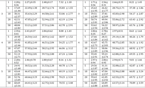
For face recognition results, the experimental results were shown in Table 1-2 for each color model. The Nearest Neighbor Classifier with the Euclidean distance measure to classify the top

P

features and my experimental results were tested up to

P



50

features in face recognition. The face recognition rates were

compared between the PCA, MPCA, SO-MPCA and SO-MPCA-RS methods and the results shown that SO-MPCA-RS outperforms the other three methods. In addition, the recognition results from SO-MPCA-RS has the highest performance especially in HSV color model.

Fig. 5. Some original high-resolution color face images from FERET (30 30 3  ) for testing.

RGB YCbCr

L P PCA MPCA SO-MPCA SO-MPCA-RS L P PCA MPCA SO-MPCA SO-MPCA-RS

1 2.45

0.33 2.410.35 2.59 0.42 6.15 1.52 1 2.240.41 2.39 0.28 2.50 0.33 6.02 1.47 5 13.12

1.48 15.241.56 16.07 1.61 28.33 2.13 5 12.571.32 15.08 1.51 15.81 1.52 28.19 2.05 1 10 19.43

2.06 20.13

1.98

21.88 2.23 37.64 3.38 1 10 18.65 1.81

20.11 2.03 21.67 2.25 37.48 3.55

20 26.85

2.31 28.172.39 30.72 2.51 41.06 3.79 20 25.732.45 28.17 2.39 30.56 2.48 40.87 3.71 Table 1. Color Face Recognition Rates in Percentage (Mean



std) on the FERET Subset of RGB and YCbCr

(7)

50 31.78

2.42 31.852.47 34.67 2.65 45.82 3.82 50 30.892.67 31.65 2.52 34.59 2.67 45.36 3.74 1 2.48

0.62 2.510.48 2.69 1.43 7.82 1.15 1 2.330.56 2.46 0.47 2.63 1.29 7.77 1.08 5 18.94

1.55 20.031.27 23.65 1.89 33.69 1.48 5 18.181.43 19.85 1.22 23.51 1.72 33.56 1.32 2 10 30.88

2.43 31.611.71 37.36 2.64 46.72 1.93 2 10 30.252.49 31.31 1.70 37.09 2.56 46.03 1.85 20 41.71

2.52 40.712.07 45.28 2.71 53.23 2.13 20 41.242.36 40.63 2.09 45.12 2.64 52.87 2.05 50 47.02

2.61 48.85

2.69

49.73 2.82 55.71 2.26 50 46.58 2.77

48.79 2.71 49.71 2.89 55.82 2.34

1 2.59

0.14 2.430.26 2.51 0.22 7.93 1.21 1 2.410.18 2.36 0.21 2.48 0.17 7.87 1.09 5 24.07

1.62 25.631.57 28.92 1.85 36.45 1.72 5 23.881.53 25.56 1.54 28.71 1.74 36.16 1.65 3 10 38.47

2.55 36.942.31 44.76 2.64 53.68 2.91 3 10 38.092.52 36.92 2.33 44.58 2.61 53.19 2.83 20 49.63

2.67 47.282.55 52.89 2.53 62.75 2.85 20 49.542.71 47.31 2.58 52.94 2.55 62.38 2.91 50 52.44

2.64 53.082.79 57.33 2.78 63.14 2.77 50 53.952.76 53.11 2.76 57.51 2.86 63.05 2.88 1 2.61

0.27 2.540.36 2.85 0.61 8.06 1.45 1 2.580.32 2.47 0.28 2.84 0.62 8.13 1.49 5 26.87

1.79 27.951.81 28.93 1.56 39.89 1.65 5 26.921.88 27.38 1.72 28.91 1.62 39.65 1.61 4 10 42.59

2.61 43.822.77 46.68 2.86 55.81 1.97 4 10 42.432.59 43.01 2.56 46.51 2.84 54.37 1.86 20 54.97

2.81 57.232.81 58.07 2.91 66.08 1 20 54.112.89 57.14 2.77 58.21 2.95 66.14 50 57.01

2.76 58.162.95 59.77 2.84 67.23 2.83 50 57.362.97 58.09 2.93 59.72 2.88 67.36 2.97 1 2.65

0.87 2.510.73 2.81 0.63 8.27 1.58 1 2.660.93 2.50 0.64 2.80 0.67 8.11 1.36 5 28.93

1.91 30.671.81 31.65 2.34 41.71 1.83 5 28.781.82 30.66 1.83 31.53 2.28 40.93 1.74 5 10 47.26

2.79 46.592.85 52.78 2.76 60.52 3.46 5 10 47.912.84 46.61 2.93 52.66 2.75 60.35 3.33 20 57.72

2.96 60.933.08 61.47 2.95 69.84 3.29 20 57.083.16 60.84 3.18 61.04 2.98 70.16 3.27 50 63.65

2.84 64.723.21 63.41 3.06 70.27 3.25 50 64.293.34 64.53 3.19 62.75 3.02 70.38 3.32

HSV CIELaB

L P PCA MPCA SO-MPCA SO-MPCA-RS L P PCA MPCA SO-MPCA SO-MPCA-RS 1 1.87

0.25 2.25 0.29 2.50 0.33 5.61 1.24 1 2.480.41 2.530.27 2.71 0.56 6.72 1.85 5 9.33

1.18 12.44 1.36 15.81 1.52 20.76 1.48 5 13.561.52 15.841.61 16.93 1.72 28.97 2.26 1 10 14.82

1.39 18.72 1.75 21.67 2.25 31.17 2.89 1 10 19.692.24 21.771.89 23.54 2.59 38.07 3.45 20 23.61

2.06 27.65 2.27 30.56 2.48 38.72 3.15 20 27.112.59 28.822.52 34.06 2.78 42.36 3.61 50 27.95

2.34 30.12 2.48 34.59 2.67 43.11 3.26 50 32.662.78 32.042.65 36.36 2.88 46.78 3.98 1 2.07

0.28 2.31 0.42 2.63 1.29 6.63 1.15 1 2.650.69 2.650.56 2.89 1.57 7.93 1.38 5 12.76

1.25 19.13 1.18 23.51 1.72 30.47 1.26 5 19.131.66 22.881.42 24.92 1.85 34.05 1.52 2 10 23.63

2.18 30.67 1.84 37.09 2.56 44.96 2.07 2 10 31.542.72 34.711.83 39.05 2.76 47.66 2.09 20 36.91

2.24

40.32 2.56 45.12 2.64 49.31 2.43 20 41.93 2.88

47.32 2.25

47.08 2.81 54.19 2.25

50 40.11 2.79

48.51 2.88 49.71 2.89 53.27 2.69 50 48.53 2.97

49.33 2.76

49.63 2.99 55.98 2.61

(8)

1 2.28

0.36 2.27 0.35 2.48 0.17 7.32 1.18 1 2.710.56 2.560.31 2.66 0.35 8.22 1.45 5 17.69

1.44 22.49 1.38 28.71 1.74 35.83 1.55 5 25.631.95 26.421.77 28.75 1.71 37.38 1.86 3 10 30.31

2.37 35.63 2.29 44.58 2.61 53.06 2.77 3 10 39.512.89 37.812.69 45.83 2.98 54.17 2.87 20 42.51

2.63 47.05 2.47 52.94 2.55 62.19 2.94 20 50.742.81 49.942.86 55.06 2.72 63.43 2.92 50 48.84

2.82 53.21 2.83 57.51 2.86 62.78 2.91 50 53.622.94 54.222.94 58.97 2.84 65.76 2.98 1 2.35

0.41

2.41 0.37 2.84 0.62 8.08 1.43 1 2.84 0.35

2.78 0.27

2.97 0.51 8.63 1.64

5 20.58

1.62 26.54 1.63 28.91 1.62 38.97 1.52 5 27.661.84 28.311.62 29.14 1.38 40.26 1.79 4 10 39.93

2.46 41.85 2.49 46.51 2.84 54.25 1.77 4 10 43.672.73 45.752.83 48.77 2.85 56.31 1.92 20 47.07

2.76 57.02 2.66 58.21 2.95 66.06 1 20 55.132.89 58.062.96 59.56 3.31 68.92 50 51.13

2.71 57.93 2.81 59.72 2.88 67.24 3.06 50 59.452.91 59.232.74 62.88 3.26 69.55 2.95 1 2.28

0.52 2.46 0.78 2.80 0.67 8.16 1.32 1 2.970.94 2.860.95 2.94 0.71 9.03 1.66 5 24.91

1.68 30.52 1.81 31.53 2.28 40.78 1.76 5 29.561.87 31.311.66 32.08 2.25 42.87 1.95 5 10 43.64

2.81 46.47 2.85 52.66 2.75 60.19 3.25 5 10 48.142.82 47.042.57 52.96 2.88 66.81 3.24 20 52.76

3.05 60.66 3.19 61.04 2.98 70.23 3.34 20 59.632.95 61.052.92 62.53 2.91 69.72 3.17 50 60.69

3.16 64.41 3.23 62.75 3.02 70.55 3.48 50 66.852.88 64.893.03 63.57 3.14 70.89 3.59

In case of the smaller L1, 2,3, MPCA and SO-MPCA methods are similar results but SO-MPCA-RS can make a good improvement over existing methods, then SO-MPCA-RS can solve the small sample size (overfitting) problem. In Table 1-2, for large L4,5, SO-MPCA-RS method is suitable for all color spaces especially in CIELaB color space.

For time performance results, I compared the execution time between our proposed method and other methods, such as PCA and MPCA in all color spaces. These experiments are performed by using a desktop-computer equipped with Microsoft Windows10 (64 bits) and an Intel(R) Core(TM) i5-7200U CPU with 2.50GHz and 4GB of RAM. In Table 3-6, the MPCA method was 0.125 – 1.349 seconds, 0.155 – 1.426 seconds, 0.179 – 1.663 seconds and 0.136 – 1.366 seconds which they were depended on no. of images and color model. However, I find that the SO-MPCA-RS required the shortest execution time of all recognition methods. The execution time from all methods in RGB color model were less than the other models and also similar to CIELaB color model. However, in HSV color model, it required the longest time of all color spaces.

No. of images PCA MPCA SO-MPCA SO-MPCA-RS 5 0.208 0.125 0.113 0.106 10 0.376 0.227 0.207 0.192 15 0.691 0.386 0.363 0.348 30 1.103 0.674 0.618 0.605 50 2.177 1.349 1.302 1.287

Table 3. Execution Time (Second) for Different Versions of the Recognition Methods in RGB Color Model

(9)

6. Conclusions

This paper proposes a novel color face recognition with Semi-Orthogonal MPCA Method. This method can capture more variance and learn more features than full orthogonality. To test our proposed method, we used color facial images from the FERET database to validate the algorithm. The experiments clearly demonstrated that SO-MPCA-RS achieves the best overall performance compared with competing methods. The complexity of proposed method which presented by execution time was shown to be less than that of the MPCA method. Then, it can be suitable for all color models. This is the next step to using the SO- MPCA for apply to each mode across different views and under changing illumination conditions.

Table 5. Execution Time (Second) for Different Versions of the Recognition Methods in HSV Color Model

Table 6. Execution Time (Second) for Different Versions of the Recognition Methods in CIELaB Color Model

References

[1] Jafri, R., & Arabnia, H. (2009). A survey of face recognition techniques.JIPS, 41-68.

[2] Zhao, W., Chellapa, R., Phillips, P. J., & Rosenfeld, A. Face Recognition: A Literature Survey. Technical Report CART-TR-948. University of Maryland.

[3] Rizk, M. R. M., & Koosha, E. M. (2006). A comparison of principal component analysis and generalized hebbian algorithm for image compression and face recognition. Proceedings of the IEEE Int. Conf. on Computer Engineering and Systems(pp. 214-219).

[4] Ke, Y., & Sukthankar, R. (2004). A more distinctive representation for local image descriptors. Proceedings of the IEEE Int. Conf. on Computer Vision and Pattern Recognition:Vol. 2. (pp. 506-513). [5] Lu, H., Plataniotis, K. N. K., & Ventsanopoulos, A. N. (2008). MPCA multilinear principal component

analysis of tensor objects.IEEE Trans. Neural Netw.,19(1), 18-39.

[6] Satone, M. P., & Kharate, G. K. (2011, March). Face detection and recognition in color images. International Journal of Computer Science Issues, IJCSI,8(2).

[7] Lukac, R., & Plataniotis, K. N. (2006). Color Image Processing: Methods and Applications. CRC Press. [8] Shashua, A. & Levin, A. (2001). Linear image coding for regression and classification using the

tensor-rank principle.Proceedings of the IEEE Int. Conf. on Computer Vision and Pattern Recognition: Vol. I. (pp. 42-49).

[9] Hua, G., Viola, P. A., & Drucker, S. M. (2007). Face recognition using discriminatively trained orthogonal rank one tensor projections. Proceedings of the IEEE Int. Conf. on Computer Vision and Pattern Recognition(pp. 1-8).

(10)

[11] Edelman, A., Arias, T. A., & Smith, S. T. (1998). The geometry of algorithms with orthogonality constraints. SIAM J. Matrix Anal. Appl., 20(2), 303-353,.

[12] Asavaskulkeit, K., & Jitapunkul, S. (2011). Generalized color face hallucination with linear regression model in MPCA. IEEE Trans. on Fundamentals of Electronics, Communications and Computer Sciences, E94-A(8), 1724-1737.

[14] Shi, Q., & Lu, H. (2015, July 25-31). Semi-orthogonal multilinear PCA with relaxed start.Proceedings of the International Joint Conference on Artificial Intelligence (IJCAI 2015) (pp. 3805-3811).

[15] Phillips, P. J., Moon, H., Rizvi, S. A., & Rauss, P. J. The FERET evaluation methodology for face recognition algorithms. IEEE Trans. PAMI 22.

K. Asavaskulkeit received the B. Eng. in electrical engineering from Department of Electrical Engineering, Chulalongkorn University, Thailand, in 2001 and the M.Eng. degree in electrical engineering from Department of Electrical Engineering, Chulalongkorn University, Thailand, in 2004. He received the Ph.D. from Department of Electrical Engineering, Chulalongkorn University, Thailand. He was appointed as a lecturer in the Department of Electrical Engineering at Mahidol University in 2011, an assistant professor in 2014. His current research interests are in image and video processing, signal compression, DSP in telecommunication.