Computer Simulation of Chaotic Systems
T. K. Genger
University of Agriculture, Makurdi
Department of Electrical and Electronics Engineering Benue State, Nigeria
T. J. Anande
University of Agriculture, Makurdi
Department of Electrical and Electronics Engineering Benue State, Nigeria
S. Al-Shehri
Swansea University,Bay Campus, Swansea Department of Electrical and Electronics Engineering
SA1 8EN, United Kingdom
ABSTRACT
This paper is about the implementation of a software tool to aid the study of chaos theory in the the context of the financial or commodities markets. The main focus of this paper is simulating the movement of oil prices in an attempt to identity chaos when it exists. Models implemented represent certain economically re-alistic aspects of the oil market. Tests for chaos (Lyapunov expo-nent test) will be conducted on these models, an attempt will be made to test for chaos in the movement of the price of oil dated from 2006 to 2016. The models implemented here are nonlinear models with the potential of exhibiting chaos for certain param-eter values. Shocks will be introduced into the models and their effect on the models will be noted and visualized through the use of a time series or graphs.
An Object oriented programming language (Java) was used in building this application, MYSQL database was used to save the data generated by the models and the spiral soft-ware development life-cycle was used in structuring, plan-ning and controlling the process of building this application.
General Terms:
Lyapunov Exponent, Chaos
Keywords
Shocks, Demand & Supply, Mean Reversion, logistic Map, Non-linear
1. INTRODUCTION
According to Ancient Chinese myth, the creators of the universe (Yin and Yang) emerged from Chaos. The ancient Greeks ac-cepted that Chaos precedes order, as written by Hesiod in his poem which states that ?first of all chaos came to be, and then the earth and everything stable”[20]. Although Chaos has always existed, it was only regarded as myth, not until the emergence of mathematical theories of chaos motion in the 20th century. At-tempts at predicting the long-term future of certain systems (this is where interacting parts assemble together) like the weather, prices of commodities and size of insect population has proved very difficult despite the presence of super computers, not be-cause these systems are computationally complex but due to their high sensitivity to initial conditions [11].This behavior is termed chaotic, because for chaotic systems, no matter how much data we accumulate about a system’s past, we cannot accurately pre-dict its future[16]. Another example of potentially chaotic sys-tems is the global financial system and commodities markets. After the market crash of October 1987, new ways of analyz-ing financial time series and applyanalyz-ing chaos theory has become an area of interest [18]. There are a number of factors affect-ing the prices in any financial system includaffect-ing the oil market,
most importantly are the global demand and supply along with some geopolitical factors. This paper focuses on modelling the existence of chaos in the financial system, the oil market in par-ticular. Several approaches exist, some of which are data driven, for example Neutral networks or autoregressive models. Chaos helps explain the irregular behavior of the oil market with time, and this is done through what is called a time series.
Linear econometric models are not suitable for the capturing the chaotic behavior of the oil market this is due to their inability to cope with the complexity of the market and the number of vari-ables that bring about changes in the price of the oil. Nonlinear models can still be deterministic.
This application simulates the Oil market, tests for the presence of chaos on real oil prices dated as far back as 2006 to March 2016. This application also simulates two different non-linear models that represent the oil market. In addition to that, this ap-plication also generates static and dynamic visualizations of that show changes in price over time.
Review
The aim of this paper is to develop a simulation of the oil mar-ket by capturing price movements in the form of a time series. Time series data is generated by the two independent models and saved in a database or the time series can be generated from his-toric data (Actual price from the OPEC). An attempt to test for chaos (Lyapunov Exponent) will be conducted on the models as well as the actual Oil data (OPEC prices). In order to achieve this, a Spiral software methodology alongside an Object oriented programming language, which in this case Java, was used in the implementation of this paper.
This application has been designed for a user who is
—An oil economics specialist.
—Not expert in maths or programming.
—A user who wishes to manipulate/research selected models that potentially demonstrate chaotic features and be able to quantitatively identify chaos when it occurs.
—In need of an application to display, calculate and save models so that they can manipulate parameters while having the pro-gram store the results for future use, allowing the user focus on the economic principles rather than maths, graphing and data management.
Challenges Encountered
(1) Model Selection: This was by far the most challenging part of this implementation, taking into account that linear econometric models neglect several constraints that affect the oil market; building simulations based linear models will not be suitable in capturing the presence of chaos. There seems to be no consensus in the literature as to what the most appropriate model of the oil market prices is. Models used in this application are nonlinear and have features that ac-curately modelled economically relevant quantities in the fi-nancial system. They are models from the literature with po-tential to display chaotic behaviour, while also having sound economic reasoning.
(2) Time series: Creating a dynamic time series was paramount in this simulation because it represented the change in price over time. Most graphing packages in Java produce static graphs, creating a dynamic time series was a rather difficult challenge to overcome. JFreeChart is a free Java chart li-brary thats supports several charts. Although it is developed as a Java package, significant time was invested in getting fa-miliarized with the necessary objects and methods required in building the static and dynamic time series.
(3) Shocks: One of the most important functionalities proposed in this application was allowing the user manipulate the time series with the intention of introducing external shocks to the system. These shocks represent events that occur in the oil market, and these events give rise to spikes or sud-den changes in average value in price of oil. Although the time these spikes occur cannot be predicted in actual cir-cumstances, this application could help in the study and un-derstanding of how changes in economic parameter values (modelled by parameters in the models) affect the movement of the price of Oil.
2. BACKGROUND RESEARCH
This section contains additional background information on the models and how they relate to the oil market. Furthermore, the connection between these models and the study of chaos and its underlying principles will be established. Finally the presence of chaos via its tests will be discussed.
An evolving system for example, f(t) under an operatorΦt, with
an initial conditionX0will not exhibit chaos if
—Φ(X0)goes to an equilibrium whent→ ∞
—Φ(X0)goes to an equilibrium whent→0
—Φ(X0)escapes to∞ast→ ∞
If the preceding statements are true, then the system does not be-have in a chaotic manner because it is predictable. If a subset of the systems orbits is confined to a bounded region but still be-haves in an unpredictable manner, this type of irregular motion can be described as chaos.
In finance, Chaos is a complex phenomenon in markets that is as a result of rapid and unsymmetrical flows of information result-ing in non-linearity in returns. Although the models proposed do not aim to precisely predict the future prices of oil, they model the oil market and capture if any, the potential of the market to exhibit chaos.
The first model simulates the price of oil as a simplified version of a mean reversion process. The second model, uses demand and supply stability analysis of an appropriate time-delayed dif-ferential equation.
Model 1: Mean Reversion
Mean reversion of a price series is a possible state when price is oscillating perhaps randomly about some unknown mean value. That is, it is not trending [1]. This model suggests that price and returns of a commodity like oil for example, tend to return back to an average price after a period of time. This average could
be the average price of oil dating back to a period in the past. Oil prices have a short term oscillation that tend to revert back to a normal long term equilibrium level. Or in the case of a cartelized commodity like oil, the long-run profit-maximizing price sought by cartel managers [14]. Evidence of mean rever-sion can be found in future markets [5], if spot prices (the im-mediate selling price of oil rather than the future [17]) are high, future prices decrease towards the normal long-run level, and in-crease if spot prices are low. In the case of volatility, which is believed to the same for both spot prices and future prices, if the prices follow a random walk, according to data, spot prices are more volatile than future prices. Work by Bembinder et al (p.373-374) [6] on mean reversion in equilibrium asset prices show that there is strong mean reversion in oil prices but it is weak in precious metal and financial assets; thus justifying the use of Mean Reverting model.
Pn+1=Pn+ηPn(M−Pn)δt+σPn
√
δtn (1)
In 1Pnis the price at timenδt,δtis the time increment. In the
case of this implementation, the time increment is 1, because the price is simulated on a daily basis.
ηis the reversion factor, the sensitivity with which the price re-verts back to the long run equilibrium mean
M is the average mean price of oil (the pricing level in which the cartel is willing to sell the product in a long term. The term
σPn
√
δtn (2)
is the continuous time uncertainty represented by volatility.nis
a random volatility effect sampled from a standard normal distri-bution.
Taking into account that the objective of the proposed application is the simulation of the oil market with special interest on the presence of chaos even without the effect of random information, I will be neglecting the final term in the equation because it adds a random behavior to the proposed model. Therefore neglecting the random effect simplifies the proposed model is follows:
Pn+1=Pn+ηPn(M−Pn)δt (3)
Model 2: Demand and Supply
The design of this model is on the basis of demand and sup-ply, taking into consideration factors affecting the movements in the supply and demand curve. Factors that are likely to cause a change in the demand curve ranges from economic crisis, in-crease in world population, politics, natural catastrophes, wars etc. While those affecting the demand curve could also be in-crease in investment that is in terms of searching for new Oil fields, ecological restrictions and so on. The supply of oil could be assumed to be from either OPEC or non-OPEC countries, the demand from the United States of America or Asia, or the entire global demand and supply.
Although the proposed model does not capture all these factors, the model attempts to capture the changes in price through the use of the elasticity of demand and supply (a change in price affects a change in the quantity of Oil demand and supplied) as well as the in-elasticity (a change in price does not have an effect on the quantity demanded or supplied). A model suggested by [15] is
Pn+1=Pn+δt.β
hα1
Pn
+α2
i
eα3n−F(P n−N)
(4)
Ignoring any explicit time dependency in demand effect (i.e. α3 = 0so that eα3n = 1) and assuming (also suggested by
Pn+1=Pn+
β.δt.α1
Pn
+(α2.β.δt+α3.βδtln 5)−β.δt.α3.lnPn−N
(5) Where; following [15] we set the fifth parameterα3, equal to
best fit value from historic data
α3=
110
3 (6)
The model can be simplified as
Pn+1=Pn+βδt
hα
1
Pn
+α2−
110 3 ln
Pn−N
5
i
(7)
where the remaining four parametersα1, α2,β and N can be
given economic interpretations α1elastic demand parameter.
α2static demand parameter.
βsensitivity parameter.
N is the significant time delay in supply due to the time frame and cost implications of exploration, infrastructure and extrac-tion process.
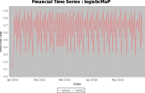
Model 3: Logistic Map
Although the logistic map does not necessarily relate to the aims and objectives of this paper, the history of the logistic map is well grounded in literature and using it could of serve as a way of testing the accuracy this application. For example, in litera-ture, certain values of r in the equation below produce Chaos and therefore a known Lyapunov exponent [7]. This value can then be compared to the Lyapunov exponent generated in this application to test its percentage accuracy.
Xn+1=r.Xn(1−Xn) (8)
This nonlinear model exhibits a range of behaviors as the value ofris varied. the Logistic map exhibits chaos for value of r = 3.65.
Fig. 1. Logistic Map where r = 3.65.
Testing For Chaos
Chaos theory is the study of unstable aperiodic behavior of deter-ministic nonlinear dynamical systems [8]. A system where none of the variables describing its state undergo a regular repetition of values is said to possess an aperiodic behavior, such systems manifest the effects of changes in its variables, this characteristic makes it difficult to predict over a long period of time intervals. The oil market has several variables that affect its current and fu-ture state, these variables like that of an aperiodic system do not
Table 1. N * mmax Dimension Embedding Matrix. P0 P1 P2 · · · Pmmax
P1 P2 P3 · · · Pmmax+1
P2 P3
. . . . . . P3 . . . . . . . . . . . . . . . . . . . . . . . . . . . . . .
PN−mmax PN
. . . . . . . . . pN . . . . . .
undergo a regular repetition of values. Studying chaotic behav-ior has the potential of explaining price fluctuations that appear to be random in the oil market. There are a number of methods that can be applied in detecting the presence of chaos in a time series, methods such as the Kolmogorov entropy, the Correlation Dimension and the Lyapunov exponent [2] [12].
The Kolmogorov entropy and the Correlation Dimension work well in theory but for this paper, only the Lyapunov exponent will be implemented.
Lyapunov Exponent
The Lyapunov exponents of a phase space are the average expo-nential rates of divergence or convergence of nearby orbits [4]. The ability to predict the state of chaotic systems is lost as or-bits that initially have identical states diverge exponentially to a point where their orbits behave quite differently. A system is termed chaotic if it contains at least one positive Lyapunov expo-nent, the time scale in which the system becomes unpredictable reflects the magnitude of the Lyapunov exponent.
Calculating The Lyapunov Exponent
In this paper, a numerical method for estimating the largest Lya-punov exponent was implemented. This is done by averaging the natural log of the growth the distance between nearest neigh-bor rows in the embedded matrix derived from the time series of length N. The method can use average growth over a selectable number of time steps.
Pi={P0, P1, ..., PN, PN+1, PN+imax} (9)
imaxis the maximum number of time-steps over which to calcu-late the growth, N+imaxis the number of iterations required to stop the algorithm from crashing.mmaxis the maximum embed-ding dimension used to construct the embedembed-ding dimension.
Xn,m=P(n+m) m= 0, ...., mmax n= 0, ...N+mmax−m
the method works by calculating the “distance” between rows
d(n, j, m) =
v u u t p=m X p=0
(Xn,p−Xj,p) 2
(10)
The algorithm below was used in identifying the “nearest neigh-bor” of each row:
(m=0; m≤mmax; m++) (i=0; i≤N-mmax; i++)
Calculate the distances d(n,j,m) for all j0, ....,(N-mmax) except j = i SetN N(n, m) =jmin wherejminis the row index such
that d(n,jmin,m) is the minimum of all distances calculated for a
The Lyapunov estimate (c.f equation(9) in Rosenstein et al.[19]) for embedding m and step size i is
L(i, m) = 1 ∆t.i
1 N−m−i
p=N−m−i
X
p=0
ln
d(p+i, N N(p, m) +i, m) d(p, N N(p, m), m)
(11) This averages, over all rows, the growth in the distance between the row and its nearest neighbor.
The Correlation Dimension
Calculating the Correlation Dimension is used in detecting the presence of chaos in experimental data. Using Grassberger and Procaccia method [1983a, 1983b], a correlation integral C(r) is constructed such that it is equal to the probability that two arbi-trary points on the orbit in a state space are closer together than r [21]. The correlation integral is computed by finding the dif-ferenceδrbetween any pair of N data points. The formula for calculating the correlation dimension is
D2= lim
∆r→0rlim→0Nlim→∞
dlog(C) dlog(r)
(12)
Apart from exceptional cases like the Lorenz model and the Henon map, the computed value ofD2 converges very slowly
[10]. Grassberger and Procaccia addressed the problems identi-fied with slow convergence and proposed a solution of embed-ding the data in a higher dimension, although their proposed so-lution was helpful, it did not solve the problem [21].
Due to this difficulty, there lacks any credible numerical calcu-lations of the correlation dimension [21]. So it is not practical to implement this method in this paper.
3. MODELING SHOCKS
A shock in the oil market with respect to price is caused by a fluctuation brought about by a sudden change in the demand side or supply side of the oil market. This sudden change in price could be as a result of several events either man made or natural, examples of such events and their corresponding effects on the price oil are.
Following the Yom Kippur war in 1974-1975 the US and global economy fell into recession this lead to a three time increase in the price of oil [13]. A shock in oil price also affected the global economy in 1980-1981 and this was caused by the Iranian revolution [13]. In 1973-1974, Nigeria encountered her first oil shock that resulted in a 600% increase in the value of Nigerias export [3].
At any given time, shocks are likely to happen, in the above mod-els, shocks are caused by step changes in the parameter values, where price jumps in response to parameter shocks. Although this is a different approach to the initial proposed approach where shocks are implemented with the use of a slider to introduce a price jump in the system. After reflection, it was felt that imple-menting shocks through jumps in parameter values offers a more natural and realistic way of implementing shocks on the system. Shocks in Model 1 will be replicated when parameters M and σundergo occasional jumps in values, while Model 2 will en-counter shocks when where are step changes in elastic supply parameterα1, inelastic demand parameterα2and sensitivity
pa-rameterβ.
4. EVALUATION & TESTING
In this section, an evaluation of the application with respect to the objectives will be carried out, tests will also be conducted on the accuracy on the Lyapunov exponent (test for chaos) as well as any system inconsistencies.
This application has undergone a series of tests by comparing values generated from independent model. The numerical values
Table 2. Empirical Calculation of the Lyapunov Exponent
Number of iteration Xn λ= log
dx(n)df
1 0.360000 0.113329
2 0.921600 1.215743
3 0.289014 0.523479
4 0.821939 0.946049
5 0.585421 -0.380727
6 0.970813 1.326148
7 0.113339 1.129234
8 0.401974 -0.243079
9 0.961563 1.306306
10 0.147837 1.035782
generated by each of the models in this application were also compared to the independent values provided, to test the accu-racy of the values generated by the models. The data generated by the Logistic Map model was tested for Chaos using the Lya-punov exponent for different values ofr, the results of the tests were compared against known experimental values to test the percentage accuracy and error. The data generated by the other two models were also tested and evaluated across different pa-rameter values using Lyapunov exponent to determine if any, the presence of chaos.
A break down of the experiments conducted on the various mod-els is presented in the next section.
Experimental Analysis
This is an analysis of the tests conducted on all three models and the results obtained. The parameter values of each model will be varied and a Lyapunov exponent test for chaos will be conducted on each set of data generated by the models. The time series generated by each model will also be generated along side the percentage error.
Lyapunov Test
In order to estimate the accuracy of the Lyapunov exponent im-plemented in this application, the Lyapunov exponent of the Lo-gistic map (Model 3) implemented in this application is going to be compared to that of known values derived for published materials. The Lyapunov exponent of an equation f(x(n)) is the average absolute value of natural logarithm of its derivatives [9].
λ= log
df dx(n)
(13)
Therefore for the logistic map atr = 4.0andXn = 0.1, the
empirical calculation of the Lyapunov exponent is:
Xn+1= 4Xn(1−Xn)
Taking the derivative of the right-hand side of the equation
4−8Xn
The following table shows the logarithm for 10 iterations.
Average= 0.697226
Therefore the value for the Lyapunov Exponent = 0.697226. Using my application( using the equation 11), the value for the Lyapunov Exponent of the Logistic map at r= 4.0 andXn= 0.1
is equal to 0.692218
Percentage error= -0.7%
Model 1: Mean Reversion Model
The Mean Reversion Model represented by the equation 3, can be rewritten as
Pn+1−Pn
∆t =ηPn(M−Pn) (14)
With the new non-linear equation it could be said that the change in price over a certain period of time∆tis sensitive to the differ-ence between the mean price and the actual price. This sensitivity is known as reversion factor(η). In theory, a change in the value ofη (reversion factor) will cause a change in the state of en-tire system. The experiments below were conducted with several values forηat 200 iterations.
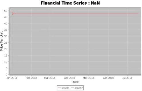
A system with a positive Lyapunov exponent(λ) can be regarded as a system exhibiting chaotic properties, according to the table above, model 1 has the potential of exhibiting chaos for values of η= 0.025, 0.0235, 0.022. therefore when the reversion factor(η) is 0.025, the rate at which the price of Oil will diverge(λ) is ap-proximately 0.067334 and so on. For values ofλ < 0, the oil market is stable and eventually reverts back to the mean price or in general terms the system reverts back to a fixed point. The time series for some of the above points are shown in figures 2 - 4
Fig. 2. Time Series Exhibiting Chaotic Behaviorλ >0
Fig. 3. Time Series whereλcould not be calculated
Fig. 4. Time Series forλ <0
Model 2: Demand and Supply Model
The demand and supply model in equation 4 can be represented in terms of demand and supply components of the model.
Pn+1=Pn+β.∆t(Dem−Sup) (15)
where Dem and Sup are the demand and supply components respectively, although the equation 15 above makes the models seem linear, this is not the case.
Pn+1−Pn
∆t =β(Dem−Sup) (16)
According to the equation 16 a change in price of Oil over a period of time∆tis proportional to a change in the difference between demand and supply components. In order words the dif-ference between demand and supply will affect price of oil over a period of time∆tand this rate of change is the sensitivity(β ). Varying the sensitivity of the model leads to changes in the state of the system, at certain values ofβthe system is can either stable, unstable or even chaotic.
Tests were conducted with different values ofβon two differ-ent computers each with a differdiffer-ent specification, it was noticed that accuracy issues began setting in at about10−13. These
ac-curacy issues where inevitable due to the limited acac-curacy of floating point storage. In chaotic time series, rounding errors be-come magnified, and this is likely to result in different Lyapunov values in different machines or implementations. The Lyapunov values obtained will always be approximate as this observation is supported in literature. The table 4 below is a subset of the data generated on one of those computers. According to the table above, the model experiences Chaos for values of sensitivity(β) equals to 2.4 and 2.3 . At these values, the rate of divergence(λ) is approximately equal to 0.601171 and 0.472365 respectively. The time series observed at certain values ofβ
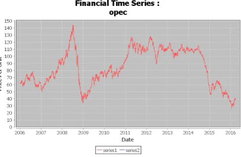
Test for Chaos On Actual Oil Data
Table 3. Lyapunov Exponents for Model 1 at 200 iterations Initial Price Mean Price Reversion Factor(η) Lyapunov Exponent (λ)
130 120 0.03 NaN
130 120 0.025 0.067334
130 120 0.0235 0.29925
130 120 0.022 0.275378
130 120 0.02 NaN
130 120 0.0167 -0.022095
130 120 0.0 NaN
130 120 1 NaN
130 120 2 NaN
130 120 3 NaN
Table 4. Lyapunov Exponents for Model 2 at 200 iterations
Initial Price Elastic Demand Static Demand Sensitivity(β) Lyapunov Exponent(λ)
110.06 900 60 2.4 0.601171
110.06 900 60 2.3 0.472365
110.06 900 60 2.0 -0.027288
110.06 900 60 1.5 -0.114167
110.06 900 60 1.0 NaN
110.06 900 60 0.5 NaN
110.06 900 60 0.3 NaN
110.06 900 60 0.1 -0.127636
Fig. 5. Time Series Exhibiting Chaotic Behavior atβ= 2.4andλ >0
Fig. 6. Time Series Exhibiting a Stable Behavior atβ= 2.0andλ <0
Shocks
In testing the effect of shocks on the application, parameters of each model was subjected to a change, and the effect was taken into account.
Fig. 7. Time Series Exhibiting an Unstable Behavior atβ = 1.0and where a sensible value forλcould not be calculated
Fig. 8. Time Series for OPEC oil prices from 2006 - 2016
Model one
Table 5. Model One Parameter Producing Chaos
Price Before Shock Price After Shock
130.00000 130.0 97.50000 109.80582 152.34375 146.56992 29.15954 64.85391 95.38120 157.32754 154.08546 28.53453 22.78360 94.37553 78.15710 161.31909 159.91509 13.62954 0.33944 50.00931
Table 6. Model Two Parameter Producing Chaos
Price Before Shock(η) After Shock Price
110.060000 110.060000 6.144021 6.708259 463.680702 437.754619 224.135368 203.467884 50.667022 39.401429 34.219715 57.418967 70.507458 26.698961 14.696391 103.281914 202.622116 6.562023 38.644203 446.550065
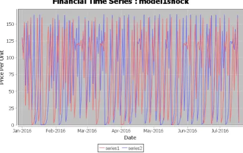
effect of a 3% increase in mean price is significant from the 3rd row of the table where there is a significant difference in the price without the influence of a shock and that with the introduction of a shock. The corresponding time series is shown below. The blue
Fig. 9. Time Series for Model one with a 3% increase in mean price
lines represent the new price as a result of the shock and the red lines is the normal price without the introduction of any shock.
Model Two
Subjecting model two to a shock means either increasing or de-creasing any of its parameters, the experiment results obtained were from an increase in the value of the Elastic Demand pa-rameter, and the extent to which this shock was encountered was recorded in the table below. The table below is for a 3% increase in the elastic demand. The table above is a subset of the entire data generated.According to the table 6 above, the effect of a 3% increase in elastic demand caused a drastic change in the system. Effect of this change can be seen from the3rdrow where the
difference between both prices is significantly high. the figure
Fig. 10. Time Series for Model Two with a 3% Increase in Elastic De-mand
above is the time series illustrating the introduction of a shock on the model, blue lines represent the new prices as a result of the shock and the red line the normal price without any shock. Finally, due to the nature of this application, any user interested in using this application will be a client looking for a bespoke application (custom application). If the client’s aims and objec-tives are satisfied. In the course of this implementation, several changes were made in order to satisfy the aims and objective of this paper, most of which are described in the design evolution, although it is not included in this paper.
5. CONCLUSION AND REFLECTIONS
The aim of this paper was to develop a computer model of chaotic systems with special interest in the financial market and specifically, the oil market. This application was built to enable a client, to manipulate or research on selected models that affected the movement of the price of oil.
In the course of this implementation, three models were success-fully built namely; the Mean reversion model, the Demand & Supply model and the Logistic Map model. Data generated by these models were saved in a database and used to test the ex-istence of chaos using the Lyapunov exponent test. The Logistic map was used to test the value and percentage accuracy of the Lyapunov exponent implemented in this application. According to the article by Lorcan Mac Manus titled “Oil Price Cycle and Sensitivity Model”, model two is described to have an unstable behavior [15], while tests conducted using the application has shown that the model two exhibits genuinely chaotic behavior with a positive Lyapunov exponent. Shocks were implemented by changing the parameter values of the mean reversion model and the demand & supply model. A dynamic time series and static time series was used to visualize changes in the models simulated. This application was implemented using a spiral soft-ware methodology along side an object oriented programming language (Java).
6. REFERENCES
[1] The Traders’ Glossary of technical terms and topics, 2008. [2] Bahram Adrangi, Arjun Chatrath, Kanwalroop Kathy Dhanda, and Kambiz Raffiee. Chaos in oil prices? evidence from futures markets.Energy Economics, 23(4):405 – 425, 2001.
[3] Eme Akpan.Oil Price Shocks and Nigeria’s Macro Econ-omy. PhD thesis, University of Ibadan, Nigeria., 2006. [4] A.Wolf, J. Swift, H. Swinney, and J. Vastano.
[5] M.P. Baker, E.S. Mayfield, and J.E. Parsons. Alternative models of uncertain commodity prices. Energy Journal, 19:115–148, January 1998.
[6] Hendrik (. Bessembinder, Jay F. Coughenour, Margaret Monroe Smoller, and Paul J. Seguin. Mean Reversion in Equilibrium Asset Prices: Evidence from the Futures Term Structure.SSRN eLibrary, 1993.
[7] Glenn Elert. Measuring chaos, 2007.
[8] James Gleick.Chaos: Making a new science. Viking, 1987. [9] J. Orlin Grabbe.International Financial Markets. Pearson
US Imports & PHIPEs, third edition, June 1995.
[10] Peter Grassberger and Itamar Procaccia. Measuring the strangeness of strange attractors. Physica D: Nonlinear Phenomena, 9(12):189 – 208, 1983.
[11] David A Hsieh. Chaos and nonlinear dynamics: application to financial markets.The journal of finance, 46(5):1839– 1877, 1991.
[12] David A Hsieh. Chaos and nonlinear dynamics: Applica-tion to financial markets.Journal of Finance, 46(5):1839– 77, December 1991.
[13] Roger Kubarych. How oil shocks affect markets.The Inter-national Economy, 2005.
[14] D.G. Laughton and H.D. Jacoby. The effects of reversion on commodity projects of different length.Real Options in Capital Investments: Models, Strategies, and Aplications, pages 185–205, 1995.
[15] Lorcan Mac Manus. Oil price cycle and sensitivity model, 2009.
[16] Masoud Mirmomeni and William Punch. Co-evolving data driven models and test data sets with the application to fore-cast chaotic time series. In2011 IEEE Congress of Evolu-tionary Computation (CEC), pages 14–20. IEEE, 2011. [17] OECD. Spot price, 2001.
[18] Alper ¨Oz¨un. Modeling chaotic behaviours in financial mar-kets. 2006.
[19] T. Michael Rosenstein, J. James Collins, and J. Carlo De Luca. A practical method for calculating largest lya-punov exponents from small data sets. Phys. D, 65(1-2):117–134, may 1993.
[20] Ziauddin Sardar and Iwona Abrams.Introducing chaos: A graphic guide. Icon Books Ltd, 2014.