A Water Calorimeter for High Energy
X-Rays and Electrons
A J Williams
Supervisors:
Dr B Planskoy (UCL)
and
Dr K E Rosser (NPL)
ProQuest Number: 10042823
All rights reserved
INFORMATION TO ALL USERS
The quality of this reproduction is dependent upon the quality of the copy submitted.
In the unlikely event that the author did not send a complete manuscript and there are missing pages, these will be noted. Also, if material had to be removed,
a note will indicate the deletion.
uest.
ProQuest 10042823
Published by ProQuest LLC(2016). Copyright of the Dissertation is held by the Author.
All rights reserved.
This work is protected against unauthorized copying under Title 17, United States Code. Microform Edition © ProQuest LLC.
ProQuest LLC
789 East Eisenhower Parkway P.O. Box 1346
A Water Calorimeter for High Energy
X-Rays and Electrons
A J Williams
Centre for Ionising Radiation Metrology
National Physical Laboratory
Teddington
Middlesex
United Kingdom TW l 1 OLW
ABSTRACT
The current primary standards at NPL for the measurement o f absorbed dose to water in
high energy photon and electron beams are graphite calorimeters. However, the quantity of
interest in radiation dosimetry is absorbed dose to water. Therefore, a new absorbed dose
to water standard based on water calorimetry has been developed for use in high energy
photon and electron beams. The calorimeter operates at 4 “C, with temperature control
being provided by liquid cooling. The sealed glass inner vessel o f the calorimeter was
designed to minimise the effect of non-water materials on the measurement of absorbed
dose. The temperature sensing thermistor probes were designed and constructed so that
glass is the only material in contact with high purity water inside the vessel. Initial
measurements o f absorbed dose to water made in 6,10, and 19 MV photons, and 16 MeV
electrons agreed, within the measurement uncertainties o f approximately 1.5% (95% c.l.),
with those determined by graphite calorimetry. These measurements confirmed the feasibility
of the calorimeter design. Significant improvements have been made to the temperature
measurement system, the water phantom and its temperature controlled enclosure since
these measurements were performed, reducing the estimated uncertainty on the
measurement o f absorbed dose to water to 1% (95% c.l.), although further work is required
CONTENTS
1. INTRODUCTION...8
1.1 CELL SURVIVAL AND THE DOSE RESPONSE R E L A T IO N ... 8
1.2 THE DOSIMETRY CHAIN ... 12
1.3 THE PRIMARY STANDARDS... 14
1.3.1 THE BASICS OF CALORIMETRY ... 14
1.3.1.1 Absorbed Dose and the heat defect ... 14
1.3.1.2 Thermal D iffu sivity... 15
1.3.2 THE X-RAY CALORIMETER... 16
1.3.3 THE ELECTRON CALORIMETER... 17
1.4 AIM OF PRESENT P R O JE C T ... 18
1.4.1 MAIN REQUIREMENTS FOR THE NPL WATER CALORIMETER... 18
1.5 WATER C A L O R IM E T R Y ... 19
1.5.1 THE DEFINITIVE WATER CALORIMETER... 19
1.5.2 THE DOMEN CALORIMETER... 19
1.6 PURE WATER CALORIMETERS... 20
1.6.1 COMPARISON OF VARIOUS WATER CALORIMETERS... 21
1.6.2 SUMMARY OF VARIOUS CALORIMETER DESIGNS ...24
1.7 NPL WATER C A LO RIM ETER... 24
1.7.1 D E S IG N ...24
1.7.2 RESEARCH PROGRAM...25
2. WATER PHANTOM AND ENCLOSURE ...27
2.1 INTRODUCTION ...27
2.2 WATER P H A N T O M ... 28
2.3 TEMPERATURE CONTROLLED ENCLOSURE ... 28
2.4 TEMPERATURE CONTROL SYSTEM AND ELECTRONICS ... 29
2.4.1 REFRIGERANT TEMPERATURE CONTROL SYSTEM ... 29
2.4.2 AIR TEMPERATURE CONTROL SYSTEM ... 30
2.5 ENCLOSURE ST A B IL IT Y ... 31
3. THE CALORIMETER V E S S E L S ... 34
3.1 DESIGN CRITERIA ... 34
3.2 METHOD OF CONSTRUCTION... 34
3.3 HEAT FLOW M O D E L L IN G ... 36
3.3.1 THE HEAT-FLOW CODE ... 36
3.3.2 CALCULATION OF THE RADIATIVE ENERGY DEPOSITION...40
3.4 CALORIMETER VESSEL SIMULATIONS ... 43
3.4.1 VESSEL TEMPERATURE PROFILES... 43
3.4.2 DIAMETER OF CALORIMETER V E SSE L S...43
3.4.3 LENGTH OF CALORIMETER VESSELS ... 45
3.4.3.1 4 to 10 M V calorimeter v e s s e l... 45
3.4.3.2 12 to 19 M V calorimeter v e s s e l...46
3.4.3.3 16 M eV Electron v e s s e l... 48
3.4.4 SUMMARY OF VESSEL EFFECTS... 51
3.4.5 SUMMARY OF VESSEL DIM ENSIONS... 51
3.4.6 CORRECTING FOR THE VESSEL EFFECT... 52
3.4.6.1 Recalculation o f the Temperature P ro files... 52
3.5 VESSEL FIT TIN G S... 57
3.6 VESSEL POSITIONING J I G ... 59
4. PRECISION TEMPERATURE MEASUREMENT S Y S T E M ... 61
4.1 SYSTEM REQUIREMENTS ...61
4.2 TEMPERATURE SENSING P R O B E S ...61
4.2.1 TEMPERATURE SENSORS... 61
4.2.2 NPL DESIGNED THERMISTOR PROBES ... 63
4.2.2.1 Construction ... 63
4.2.3.1 Thermistor Probe Temperature P rofiles... 65
4.2.3.2 Thermistor Probe Temperature Corrections...68
4.2.4 SELF-HEATING OF THERMISTOR PROBES... 70
4.3 ELECTRONICS... 71
4.3.1 BRIDGE TH EO RY...72
4.3.2 D.C. WHEATSTONE BRIDGE... 73
4.4 SYSTEM CALIBRATION... 75
4.4.1 CALIBRATION METHOD... 75
4.4.2 STABILITY OF MEASUREMENT SYSTEM THERMISTOR CALIBRATIONS . . 76
5. THE HEAT D E FE C T ... 80
5.1 RADIATION CHEMISTRY ... 80
5.2 DETERMINING THE HEAT D E F E C T ... 81
5.2.1 COMPUTER SIMULATION AND RELATIVE MEASUREMENT ... 81
5.2.1.1 Literature Review ... 82
5.2.1.2 Pure water (with and without gas space) ... 83
5.2.1.3 H2 saturated w a te r... 84
5.2.1.4 H2/O2 saturated water (with gas space) ... 85
5.2.1.5 H /O2 saturated water (without gas s p a c e )... 85
5.2.2 ABSOLUTE MEASUREMENTS ... 86
5.3 D ISC U SSIO N... 87
5.4 NPL GAS FLOW SYSTEM (SINGLE GAS) ... 87
6. COMPARISON OF THE WATER CALORIMETER WITH THE NPL PRIMARY STANDARD GRAPHITE CALORIMETERS... 89
6.1 ABSORBED DOSE TO WATER DETERMINED USING GRAPHITE CALORIMETRY. ... 89
6.1.1 HIGH ENERGY PHOTON BEAMS ... 89
6.1.2 HIGH ENERGY ELECTRON B E A M S ... 90
6.2 ABSORBED DOSE TO WATER DETERMINED USING WATER CALORIMETRY. ... 91
6.2.1 HIGH ENERGY PHOTON BEAMS ...91
6.2.2 HIGH ENERGY ELECTRON B E A M S ... 93
6.3 DATA A N A L Y S IS ... 94
6.3.1 ION CHAMBER MEASUREMENTS... 94
6.3.2 CALORIMETER MEASUREMENTS... 95
6.3.3 CALCULATION OF THE CHAMBER CALIBRATION FACTOR... 97
6.3.4 CORRECTION FACTO RS... 97
6.3.4.1 H eat-fiow... 97
6.3.4.2 Density o f w a ter... 98
6.3.4.3 Perturbation o f the radiation beam ... 98
6.4 R E S U L T S ... 99
6.4.1 CALORIMETER STABILITY ... 99
6.4.2 CALORIMETER MEASUREMENTS... 102
6.4.3 CHAMBER MEASUREMENTS... 103
6.4.4 CHAMBER CALIBRATION FACTORS... 104
6.5 UNCERTAINTIES... 107
7. DISCUSSION ... 110
7.1 DEVELOPMENTS TO OCTOBER 1998 ... 110
7.2 FURTHER INVESTIGATIONS ... 110
8. A N E W WATER PHANTOM AND ENCLOSURE... 112
8.1 PROBLEMS WITH THE PREVIOUS S Y S T E M ... 112
8.2 THE NEW P H A N T O M ... 113
8.3 THE NEW E N C L O SU R E ... 114
8.4 WATER FLOW IN THE PHANTOM ... 115
8.5 TEMPERATURE CONTROL SYSTEM ... 116
8.6 TEMPERATURE CALIBRATION OF CONTROL S Y S T E M ... 119
9. AN A.C. TEMPERATURE MEASUREMENT SYSTEM ... 122
9.1 A.C. B R ID G E ... 122
9.1.1 THEORY... 122
9.1.2 DESIGN AND CONSTRUCTION... 122
9.1.3 The L IA ... 126
9.1.3.1 The thermistor p r o b e s... 127
9.1.3.2 The R e s n e ts... 127
9.1.4 OPTIMIZATION OF THE A.C. BR ID G E... 128
9.1.4.1 Bridge Drive V oltage... 128
9.1.4.2 Bridge Drive Frequency ... 128
9.1.4.3 F ilte r s... 130
9.1.5 A C. BRIDGE TEST METHODS ... 130
9.1.6 TEST RESULTS... 131
9.1.6.1 Long term stability - with precision resistor in place o f therm istor 131 9.1.6.2 Bridge sensitivity and signal-to-noise ratio - with precision resistor . . . . 132
9.1.6.3 Bridge sensitivity and signal-to-noise ratio - with one thermistor probe . . 132
9.1.6.4 Bridge sensitivity and signal-to-noise ratio - with two thermistor probes . 136 9.1.7 COMPARISON OF A.C. TEST R E SU L TS... 136
9.2 D.C. B R ID G E ... 138
9.2.1 D.C. BRIDGE TEST METHODS ... 138
9.2.2 TEST RESULTS... 139
9.2.2.1 Long term sta bility... 139
9.2.2.2 Sensitivity and signal-to-noise... 140
9.3 SUMMARY OF R E S U L T S ... 141
9.4 TEMPERATURE CALIBRATION OF THE B R ID G E S ... 141
9.4.1 CALIBRATION OF D C. BRIDG E... 142
9.4.2 CALIBRATION OF A C. BRIDG E... 142
10. MEASUREMENTS USING ‘®Co RADIATION... 144
10.1 SUMMARY OF R E S U L T S ... 146
11. DISCUSSION ... 147
11.1 CALORIMETER PERFORMANCE ... 147
11.2 FUTURE W O R K ... 148
11.2.1 HEAT-FLOW CORRECTIONS... 148
11.2.2 HEAT DEFECT ... 148
11.2.3 SPECIFIC HEAT CAPACITY OF WATER ... 148
11.2.4 TESTS FOR CONVECTION... 149
11.2.4.1 Thermistor p o w e r... 149
11.2.4.2 Operating temperature ... 149
11.3 CONCLUSION... 149
12. ACKNOWLEDGEMENTS ... 150
13. R E FE R E N C E S... 151
14. APPENDIX A ... 158
FIGURES Figure 1 Cell survivability curve... 8
Figure 2 The dose response relation ... 10
Figure 3 Clinically established dose-response relations... 11
Figure 4 The steps required to determine absorbed dose to the patient... 12
Figure 5 The dissemination of the High Energy Photon Absorbed Dose standard ... 13
Figure 6 Primary Standard X-ray Calorimeter... 16
Figure 7 Primary Standard Electron calorimeter... 17
Figure 9 The volume expansion coefficient of w a te r ...27
Figure 10 Schematic diagram of temperature controlled enclosure ... 29
Figure 11 Schematic diagram of refrigerant control system ... 30
Figure 12 Schematic diagram of the air control system ... 31
Figure 13 Temperature stability of enclosure... 32
Figure 14 Photograph of an X-ray calorimeter vessel ... 35
Figure 15 1-D heat-flow model - for the case all dz equal ... 36
Figure 16 1-D heat-flow - for the case unequal d z... 37
Figure 17 Finite element grid s i z e s ... 38
Figure 18 Contour plot of absorbed dose in the water phantom (without glass v e s s e l)... 41
Figure 19 Contour plot of absorbed dose in the water phantom (with glass vessel) ...41
Figure 20 Depth-dose curves for 19 MV photons in w ater...42
Figure 21 Radial dose curves for 19 MV photons in water ... 42
Figure 22 Calculated radial temperature profiles...44
Figure 23 (Calculated radial temperature profiles...44
Figure 24 Effect of vessel walls on temperature at the measurement p oin t...45
Figure 25 Calculated axial temperature profile of 4 to 10 MV calorimeter vessel ... 45
Figure 26 Axial temperature profile of the 4 to 10 MV vessel in a 16 MV photon beam ...47
Figure 27 4 to 10 MV and new vessels in 16 MV photons...47
Figure 28 Axial temperature profile of the 12 to 19 MV vessel in 16 MV photons ... 48
Figure 29 Radial temperature profile of 10 cm diameter calorimeter v e s s e l... 50
Figure 30 Axial temperature profile o f 16 MeV electron v e s s e l... 50
Figure 31 Effect on measured temperature rise of excess h e a t ... 51
Figure 32 Comparison of vessel temperature profiles at 10 M V ...52
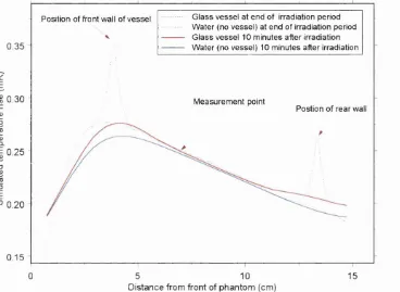
Figure 33 Temperature profiles of glass calorimeter vessel in stirred phantom ...53
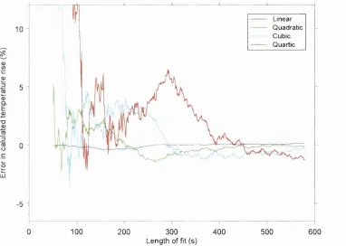
Figure 34 Temperature at measurement point against time after irradiation in stirred phantom 53 Figure 36 Error in calculated temperature rises... 55
Figure 37 Calculated temperature rise using different types of data fitting on noisy data 2 ...56
Figure 38 Side profile of the 4 to 10 MV calorimeter vessel ... 58
Figure 39 4 to 10 MV X-ray vessel - front p r o file ... 58
Figure 40 Thermistor adjustment ... 59
Figure 41 Vessel positioning jig - front v ie w ... 60
Figure 42 Vessel positioning jig - side view ... 60
Figure 43 Two types o f thermistor bead suitable for water calorimetry ... 63
Figure 44 Domen Palmans and NPL probe d esign s... 64
Figure 45 NPL thermistor p ro b e... 65
Figure 46 Thermistor probe heat-flow geom etry...66
Figure 47 Thermistor probe temperature deviations ...67
Figure 48 Temperature profile of thermistor probe ... 67
Figure 49 Error in measured temperature r is e ... 69
Figure 50 Error in measured temperature r is e ... 69
Figure 51 Thermistor self-heating... 70
Figure 52 A basic bridge circuit ... 72
Figure 53 Graphite calorimeter d.c. b r id g e ...74
Figure 54 Water calorimeter double d c. bridge...74
Figure 55 Thermistor calibration set-up ... 76
Figure 56 Plot of PRT temperature and out-of-balance bridge v o lta g e...77
Figure 57 Plot of PRT temperature against bridge voltage...77
Figure 58 Temperature measurement system calibration sta b ility ... 78
Figure 59 Temperature measurement system calibration curves for a single thermistor p ro b e 78 Figure 60 Simulation of differential exothermicity for various H2/O2 mixtures ... 86
Figure 61 The gas saturation system used at N P L ... 88
Figure 62 Graphite calorimetry derived chamber calibration fa c to rs...90
Figure 63 Graphite calorimeter derived chamber calibration fa c to rs... 91
Figure 64 Schematic diagram of X-ray beam experimental set-up... 92
Figure 65 Schematic diagram of electron beam experimental se t-u p ... 93
Figure 66 Temperature rise calculation for a typical 16 MV calorimeter r u n ... 96
Figure 67 Calorimeter to monitor ratios for 6 MV p h o to n s... 100
Figure 69 Calorimeter to monitor ratios for 16 MV p h o to n s... 101
Figure 70 Calorimeter to monitor ratios fo 16 MeV electron s... 101
Figure 71 Ratios of water to graphite calorimetry-derived chamber calibration factors ... 106
Figure 72 Ratios of water to graphite-calorimetry derived chamber calibration factors ... 106
Figure 73 The original phantom and enclosure... 112
Figure 74 New phantom: cross sectional side v i e w ... 113
Figure 75 New phantom enclosure ... 115
Figure 76 Refrigerant flow in the phantom ... 117
Figure* 77 Schematic diagram of old and new monitoring and control systems ... 118
Figure 78 Screen shot from enclosure temperature control program ... 119
Figure 79 Calibration of temperature control system probes ... 119
Figure 80 Phantom temperature stability over a 10 day period ... 121
Figure 81 Measuring assembly overview (a.c.) ... 123
Figure 82 A bridge circuit with screening to reduce capacitive pick-up... 123
Figure 83 Actual screened bridge circuit... 124
Figure 84 19" rack bridge enclosure showing the inner enclosure and connector cabling... 124
Figure 85 The iimer enclosure ... 125
Figure 86 A C . bridge sy stem ... 125
Figure 87 New wiring to thermistor probes... 127
Figure 88 Precision R e sn et... 128
Figure 89 Fourier transforms of a.c. bridge output ... 129
Figure 90 Long term stability of bridge output voltage for various drive frequencies... 131
Figure 91 21 Hz bridge output test ... 133
Figure 92 21 Hz bridge output test using a single thermistor p rob e... 134
Figure 93 32IHz bridge output test using two thermistor p rob es... 135
Figure 94 Fourier transforms of bridge output signal at 21.2 H z ... 138
Figure 96 d.c. bridge output test using a precision resistor ... 140
Figure 97 Conversion of d.c. bridge voltage versus temperature data into resistance... 142
Figure 98 Typical bridge outputs for a 2 minute ®°Co irradiation... 144
Figure 99 Comparison of a.c. and d.c. bridges in ^ C o ... 145
TABLES Table 1 Comparison of four different calorimeter d esig n s... 23
Table 2 Advantages and disadvantages of four different water calorimeter d esig n s... 24
Table 3 Inputs required for heat-flow code... 38
Table 4 Summary of vessel dimensions... 51
Table 5 Correction factors for vessel heat-flow... 57
Table 6 Peak excess temperature of thermistor probe for various doses and dose-rates...68
Table 7 Corrections factors for thermistor probe excess heat effect...70
Table 8 Calculated heat defect v a lu e s ... 82
Table 9 Abbreviated reaction scheme for pure w a ter... 84
Table 10 Abbreviated reaction scheme for H2/O2 w a te r ... 85
Table 11 Graphite calorimetry derived chamber calibration factors... 89
Table 12 Graphite calorimetry derived chamber calibration factors...91
Table 13 Experimental parameters for X-ray production...92
Table 14 Dependency of calculated temperature rise on the data fitting t y p e ... 97
Table 15 Correction factors for temperature variation in water density... 98
Table 16 Calorimeter to monitor ratios for all beam energies/qualities ... 102
Table 17 Corrected chamber to monitor ratios for all beam energies/qualities... 103
Table 18 Chamber calibration factors calculated for each measurement set at each beam energy . . . 104
Table 19 Chamber calibration factors (weighted) ... 105
Table 20 Ratio of water calorimetry derived chamber calibration factors with graphite calorimetry derived chamber calibration factors... 105
Table 21 i-distribution table - values oïk^^ ... 107
Table 22 Calculation o f uncertainties ... 108
Table 23 Final uncertainties in absorbed dose to water measurements... 109
Table 25 Bridge sensitivity calculated using a 10 kQ precision resistor... 133
Table 26 Bridge sensitivity calculated using a single 10 kQ thermistor p ro b e... 134
Table 27 Bridge sensitivity calculated using two 10 kQ thermistor probes ... 135
Table 28 LIA settings for best results... 137
Table 29 Comparison of d.c. long term stability ... 140
Table 30: d.c. bridge sensitivity calculation r e su lts... 141
Table 31 Summary of results for the comparison of a.c. and d.c. bridges... 141
Table 32 Results from a.c. and dc. bridge comparison in ^Co radiation... 145
Table 33 Model III: reactions and rate constants (25 °C)... 158
1.
INTRODUCTION
Radiotherapy treatment uses ionising radiation to destroy cancerous tissue, the aim being
to kill the tumour whilst leaving the surrounding tissue as undamaged as possible. According
to Brahme [1], ‘An absolutely necessary prerequisite for precise radiation therapy ... is a
high accuracy in the delivery o f absorbed dose [the mean energy deposited per unit mass]
to the target volume’. Brahme [1] states that the level of accuracy required depends on the
‘dose response relation’ for the tumour in question. In order to better appreciate the
requirement for accurate absorbed dose dehvery, it is advantageous to understand a simple
radiobiological model o f cell survival.
1.1 CELL SURVIVAL AND THE DOSE RESPONSE RELATION
The following model is based on that developed by Brahme [1]. The fraction of tumour
cells, S, surviving a single irradiation of absorbed dose Z), is given by a cell survival curve
such as that shown in Figure 1.
A simple approximation of the value
o f S for a given dose Z), is
^ 0.1 0
-Dose (Gy)
S = exp A
Z). (1)
Figure 1 Cell survivability curve. The fraction of cells
surviving decreases as the absorbed dose increases.
where Dq is the absorbed dose required
to reduce the proportion of surviving
tumour cells to e '\
Equation (1) can be used to calculate
the number o f tumour cells surviving
after a number o f irradiations. In this
approximation, the irradiations or
“fractions” are of equal dose (it can also
be calculated for the case when the
number o f fractions is constant and the
dose per fraction changes). If it is
assumed that tumour cells are, (i) of equal sensitivity, (ii) uniformly distributed over the
between irradiations, then the number of surviving tumour cells N(n) after n irradiations is given by
iV («)= A T (0 )n 5 '(Z ),) (2)
where N(0) is the original number of cells in the tumour. Evaluating the product in equation
(2) using equation (1) for S(D), N(n) becomes
D
Do (3)
N(n) = N(Q) exp
where
£ » = Î Z ) , (4)
;=1
i.e., net cell survival is directly proportional to the total dose D. The probability o f tumour
control, also called the dose response relation, is given by
P(D) = exp[- # (» )] (5)
and is plotted in Figure 2 for a number o f different N(0). Brahme's value for of 2.73 Gy
was used. From Figure 2, it is clear that an increase in tumour size requires an increase in
dose for the same probability of tumour control. The steepest point or gradient of these dose
response curves can be found when P(D) = e '\ However, a more useful parameter in
radiation therapy is the normalized dose response gradient y given by
dP
r = D — (6)
It describes how the tumour control probability increases with a given relative increase in
dose. In the above model, where the dose per fi-action has been kept constant, the value of
y is given by
, = M W m
e
so for the three cases in Figure 2, y = 4.2, 5.9 and 7.6 respectively. Therefore, a relative
uncertainty in the absorbed dose of 5% results in a relative uncertainty in tumour control
0.8
o c
8
3 O
E -2
"o
3-0.4 - 1/e Y = 4,2 Y = 5.9 Y = 7.6
CL
0.2
-N ( 0 ) = 10^ N ( 0 ) = 10^ N ( 0 ) = 10^
0.0
20 30 40 50 60 70
D o s e (Gy)
Figure 2 The dose response relation for 10^ 10^ and 10^ tumour cells as given by equation
(5). The curves are sigmoidal in shape, shifted to increasing dose with tumour size. The
steepest points of each curve corresponds to when P(D) = e
Brahme [ 1 ] compared the values of y calculated from the above model with those of
clinically observed gradients and found that they were similar for small tumours in the head
and neck. However, he found that for larger tumours clinically observed gradients were
generally significantly lower. The main reason for the discrepancy was the initial
assumptions set out on page 8, in particular the assumption of a perfectly uniform cell
population.
From Figure 2 it is clear that almost any tumour can be controlled given a high enough
radiation dose. However, radiation damages normal tissue as well as the tumour and in
clinical radiotherapy it is the need to control damage to normal tissue that limits the
radiation dose to the tumour. The normal tissue dose-response relation is similar in shape
to the tumour control dose-response relation, although in most cases it tends to be less
steep. The normal tissue dose-response relation must lie to the right of that for the tumour
control in order to be able to treat a tumour at all - ideally it would be well separated from
the tumour control dose-response.
Figure 3 shows clinically established tumour and severe normal tissue damage dose-
response relations for advanced head and neck tumours, taken from Aaltonen et al [2].
Aaltonen found that the clinically optimum dose for treatment of this type of tumour was
Probability o f tumour control Clinical data
Probabilty o f s e v e r e normal tis s u e d a m a g e Clinical data
Probability o f cure wittrout s e v e r e co m p lica tio n s Clinical data
0.8
"Clinically Optimal" P rescribed d o s e « 5 9 Gy T o lera n ce ran g e ± 1 Gy
0.6
-0.4
0.0
0 20 40 60 80 100
Dose (Gy)
Figure 3 Clinically established dose-response relations for advanced head and neck
tumours. The absorbed dose should be within 1 Gy of the optimal dose so as to not
loose more than 5% of patients that can be potentially cured without severe
complications.
approximately 59 Gy. Irradiation within ±1 Gy (1.7%) of this optimum dose ensures that
no more that 5% of the patients who potentially can be cured without severe complications
are lost.
Tumour normalized response gradients as high as y = 5 can be expected clinically and
gradients of y = 3 are common. Brahme [1] states that in these cases, ‘uncertainty in the
delivery of adsorbed dose would result in an increase in the number of patients suffering
from complications and recurrences due to over- and under-dosage, respectively... and for
normalized dose gradients of y = 5, ‘the total standard deviation in the dosimetry should be
less than 5%’. Additionally, in order to have a reasonable control of the treatment outcome,
Brahme suggests that the relative uncertainty in the target volume should be as small as 3%
when the normalized response gradient, y, is higher than 3. Mijnheer et al [3] proposed that
the combined uncertainty in the delivery of absorbed dose should be 3.5% given as one
relative standard deviation. Mijnheer estimated the uncertainties in a simple X-ray treatment
and found that his proposed accuracy in the delivery of absorbed dose could not at that time
be achieved. However, he stated that “This requirement of 3 .5%, which lies just beyond the
present possibilities of radiation therapy, might act as a stimulus to improve the dosimetric
techniques.”
1.2 THE DOSIMETRY CHAIN
The determination of the absorbed dose to a tumour within an irradiated patient involves
a number of steps as shown in Figure 4, adapted from Wittkamper [4],
C a l i b r a t i o n o f U s e r io ni za t io n c h a m b e r
a t N P L
A b s o r b e d d o s e a t r e l e v a n t p o in t s in a p a t i e n t u n d e r t r e a t m e n t c o n d i t i o n s
R e l a t i v e d o s e di s tr i b ut io n in a w a t e r p h a n t o m u n d e r clinically r e l e v a n t c o n d i t i o n s
A b s o r b e d d o s e d is tr i b u ti o n in a n a n t h r o p o m o r p h i c p h a n t o m u n d e r t r e a t m e n t c o n d i t i o n s
A b s o r b e d d o s e a t a r e f e r e n c e p o in t in w a t e r u n d e r
r e f e r e n c e c o n d i t i o n s
M J x , y , z ) M J r e f )
p h a n to m
' p a tie n t
Figure 4 The steps required to determine absorbed dose to the patient. The uncertainty on the
measurement of absorbed dose increases with each step.
1. Calibration of hospital ionization chamber
The first step is the calibration of a device, called an ionization chamber, used by the
hospital to determine the absorbed dose imparted by the ionising radiation output of the
treatment device, for example, a linear accelerator.
The calibration of the hospital (also called User) ionisation chamber must be traceable
to the Primary Standard for Absorbed Dose to Water. It is not practical for all the User
ionisation chambers in the United Kingdom to be calibrated directly against the UK Primary
Standard that is held at the National Physical Laboratory (NPL). Instead, the User chambers
obtain their calibration via a dissemination chain as shown in Figure 5. The example shown
is for the dissemination of the High Energy Photon Absorbed Dose to Water Standard. NPL
Primary standard
z Working
stan dards
Î
— - —
Secondary standard
Secondary standard
Secondary standard
3 Tertiary Tertiary Tertiary Tertiary Tertiary Tertiary 1 standard standard standard standard standard standard
Figure 5 The dissemination of the High Energy Photon Absorbed Dose standard. NPL
‘Working Standard’ ionization chambers are calibrated against the Primary Standard. User
chambers from hospitals that hold Secondary Standards are calibrated against the NPL
Working Standards. User chambers from hospitals that hold Tertiary Standards are calibrated
against Secondary Standard chambers.
calibrates a number of its own ionisation chambers (called Working Standard chambers)
against the Primary Standard. User ionisation chambers from a subset of UK hospitals that
hold Secondary Standards are calibrated against the NPL Working Standard ionisation
chambers. These chambers are then used to calibrate the ionisation chambers from a larger
subset of United Kingdom hospitals that hold Tertiary Standard chambers, and so on.
2. Absorbed dose to water under reference conditions
Using the chamber calibration factor given by NPL, the absorbed dose to water at the
reference depth in a water phantom is calculated under reference conditions.
3. Relative dose distribution in water
The relative dose distribution in a water phantom is measured. These measurements will
be made for beam geometries that are likely to be encountered clinically, for example, square
collimated fields of various sizes with and without beam wedges.
4. Relative dose distribution in anthropomorphic phantom
The dose distribution is measured in an anthropomorphic phantom under clinical
conditions. Y \ in Figure 4 is the product of phantom related correction factors such
as phantom inhomogeneity and contour correction.
5. Relative dose distribution in patient
The absorbed dose distribution in the patient is then determined under clinical conditions,
n ^patient ^ Figu^e 4 is the product o f patient correction factors such as patient movements during irradiation.
At each step o f the calibration chain, the uncertainty on the measurement will increase
in size. The uncertainty at the end o f step 5 is likely to be greater than 3.5% [5]. So as not
to contribute to the total uncertainty, the uncertainty on the calibration of the Secondary
Standard chamber issued by NPL should be insignificant compared to the overall final
measurement uncertainty.
1.3 THE PRIMARY STANDARDS
The present UK primary standards for both high energy X-rays and electrons at
radiotherapy level dose-rates are graphite calorimeters. Before describing these calorimeters,
it is useful to understand their basic operating principles.
1.3.1 THE BASICS OF CALORIMETRY
1.3.1.1 Absorbed Dose and the heat defect
A calorimeter is a device used to measure energy input (as heat) by measuring the
temperature rise in a known mass o f material such as water or graphite. The relationship
between absorbed dose to the medium D„ and the measured temperature rise A T is given
by
D„ = c ^ ^ T - ^
(10)where Cp is the specific heat capacity of the medium and is the heat defect (the difference
in the energy deposited and that appearing as heat). For graphite, ^ is zero, so equation
(10) reduces to
= c / r
(11)
where is the absorbed dose to graphite. For water, the heat defect is non-zero. Chapter
5 starting on page 80 has more detailed information on the heat defect but, briefly, radiation
reactions are predominantly exothermic; the opposite is true when the reactions are
predominantly endothermie. The heat defect is given by
where is the energy absorbed and Ef, is the energy appearing as heat. It is positive for
endothermie chemical reactions and negative for exothermic chemical reactions.
Graphite has a specific heat capacity o f 0.72 J.g'^K'^ at 20 C, so for a typical dose of
1 Gy, the temperature rise in graphite is 1.4 mK. The specific heat capacity o f water at
4.2 J.g'^K'^ is almost six times higher than that o f graphite, therefore the measured
temperature rise in water for an absorbed dose o f 1 Gy is just 0.23 mK.
1.3.1.2 Thermal Diffusivity
The thermal dififiisivity of a medium effects how quickly a temperature distribution will
deviate from its initial value. For example, in ^Co radiation at depths beyond the peak of
the depth-dose curve, Ross [6] showed that the time A/ taken for the temperature to change
by AT can be approximated by
1 AT
T
A f » — y — (13)
where a is the thermal diffusivity and p is the linear attenuation coefficient. The aim in
calorimetry is to measure AT to better than 0.5% therefore this requires t h a t - ^ < 0.005.
Inputting values o f a for graphite and water of 0.80 cm^.s'^ and 1.41 x 10'^ cm^.s'\ and p
of 0.05 cm'^ gives values for Et o f 2.5 s and 1400 s respectively. 2.5 s is not long enough
to complete an irradiation (a typical irradiation in X-rays lasts for 60 s). Therefore graphite
calorimeters such as the present NPL primary standard X-ray graphite calorimeter require
complex thermal isolation systems to enable measurements to be made of dose at a point.
However, in water, dose measurements can be made at a point without the need to isolate
thermally a section of the water as the energy deposited by the radiation tends to stay where
1.3.2 THE X-RAY CALORIMETER
The High Energy X-ray Graphite Calorimeter, which measures absorbed dose to graphite
at therapy level dose-rates down to 1 Gy.min'^ for X-ray energies between 4 and 19 MV,
has been in use at NPL since 1988 [7]. It was built to a design by Domen and Lamperti [8]
with modifications by Cross [9]. A simplified schematic diagram of the calorimeter is shown
in Figure 6. The calorimeter consists of a small 2.7 mm thick by 20 mm diameter disc shaped core of graphite surrounded by three graphite jackets and an extensive graphite
phantom. The jackets and phantom present a nearly homogeneous graphite medium for the
absorption and scattering of the X-ray beam. The temperature rise in the core is measured
by a 2 kfl thermistor connected to an a.c. bridge, calibrated by comparing the temperature
rise from electrical heating of the core with that of the radiation beam. Because of the small
temperature rise in the calorimeter (1.4 mK per Gy), the heat transfer between the core and
its surroundings has been minimized. Convection has been prevented by evacuating the small
gaps between the core and the jackets. Thermal radiation has been reduced by applying
Graphite phantom
Jacket 3
Jacket 2 ■ Jacket 1
Core
Build up plates
Vacuum housing
Figure 6 Primary' Standard X-ray Calorimeter. The calorimeter consists of a
small disc-shaped graphite core surrounded by three graphite jackets and an
extensive phantom. Heat transfer between the core and jackets has been
minimized by evacuating the gaps and applying aluminized Mylar films to some
components. Graphite plates are added to the front of the calorimeter to provide
build up as required.
aluminized Mylar films to the surfaces of some components. Heat conduction has been
reduced by using small polystyrene pegs to support the components.
As the calorimeter measures absorbed dose to graphite, this has to be converted into
absorbed dose to water using the formalism developed by Burns [10]. The uncertainty on
the measurement of absorbed dose to water is 1.4% (95% c.l.)
1.3.3 THE ELECTRON CALORIMETER
An electron calorimeter has been in use at NPL since 1988 [11], [12] capable of absorbed
dose to graphite measurements at high electron dose-rates (greater than 100 Gy.min'^) and
at energies above 8 MeV. However, it is only recently that a new design of electron graphite
calorimeter has been built which enables absorbed dose measurements to be made near
therapy level dose-rates and doses [13] (about 5 Gy.min'*), and at energies from 4 MeV.
The calorimeter is shown schematically in Figure 7.
E nj
c
2
■G0) lU
1 5 0 m m
T h e r m is to r
1 5 0 m m
►
/
Side view Front view
D C B rid ge
%
i ' " ’\ 4
1 .4 V
P o l y s t y r e n e b e a d s
C o r e 2 m m thick
Figure 7 Primai}^ Standard Electron calorimeter. The calorimeter consists of a small disc
shaped core surrounded by a graphite bod\'. The core is thermally isolated from the body by
a 1 mm air gap and is supported by small expanded polystyrene beads. Graphite plates are
added in front and behind the calorimeter body to provide build up and backscatter
respectively as required.
The calorimeter consists of a small graphite core surrounded by a graphite body. The
core is a disc 50 mm in diameter and 2 mm thick, surrounded by graphite body 150 by
150 mm in cross section and 6 mm in thickness. The temperature rise in the core is
measured by a 22 kfl thermistor connected to a d.c. bridge, calibrated directly in terms of
temperature against NPL temperature standards. The core is thermally isolated from the
surround by a nominal 1 mm air gap at all faces and is supported by small expanded
polystyrene beads. Graphite plates are added in front o f the calorimeter body to position the
core at the desired measurement depth and also added to the rear to provide backscatter.
The entire calorimeter assembly is enclosed in 25 mm of expanded polystyrene to provide
a degree of thermal isolation. By working at a dose rate above 5 Gy.min'^ with short
irradiations i.e., 20 s irradiations leading to temperature rises o f about 2 mK, the need for
a complex temperature control and vacuum system within the calorimeter can be obviated.
This calorimeter forms the measurement base for a calibration service for electron beam
radiotherapy which gives users ion chamber calibration factors in terms o f absorbed dose
to water. However, as the calorimeter measures absorbed dose to graphite, this has to be
converted into absorbed dose to water using a formalism developed by Bums et al
[14], [15].The uncertainty on such a calibration o f absorbed dose to water is 1.5% (95%
c.l.).
1.4 AIM OF PRESENT PROJECT
Using the current primary standard graphite calorimeters to calculate absorbed dose to
water has an obvious disadvantage in that the calorimeters actually measure absorbed dose
to graphite. The conversion from absorbed dose to graphite to absorbed dose to water
introduces significant uncertainties [10], [14] and is the principle disadvantage of graphite
calorimetry for determining absorbed dose to water. It would be advantageous if absorbed
dose to water was measured directly, using a water calorimeter, since this would avoid
introducing such uncertainties. The aim of this project was to design and build a water
calorimeter for use in high energy X-ray and electron beams which would enable ionisation
chambers to be calibrated directly in terms o f absorbed dose to water.
1.4.1 MAIN REQUIREMENTS FOR THE NPL WATER CALORIMETER.
The main requirements o f the water calorimeter to be built at NPL were that it could be
used:
• with horizontal radiation beams;
• at measurement depths of 3.3 cm (16 MeV electrons) [16] and 5 cm and 7 cm (high
energy X-rays) [17], the depths being defined by the relevant radiation Code of
• at dose-rates of between 1 Gy/min (high energy X-rays) and 16 Gy/min (16 MeV
electrons).
1.5 W ATER CALORIM ETRY
1.5.1 THE DEFINITIVE WATER CALORIMETER
If it were possible to build the ‘definitive water calorimeter’, it would consist of a mass
o f pure water with a zero heat defect, into which an infinitesimally small temperature sensor
was placed. It would be thermally isolated from its surroundings, there would be no heat
flow or convection in the water that would upset the temperature stability of the system,
there would be no containment vessel which could contaminate the water or effect the
temperature stability and no chemical impurities in the water that would result in a heat
defect.
Unfortunately, it is impossible to build the ‘definitive water calorimeter’ as described
above: liquid water has to have some kind o f containment vessel. Even using water in the
form o f ice [18] as the absorbing medium does not help because this introduces more
problems than it solves - for example, the heat defect o f ice is an unknown quantity.
Nevertheless, using a liquid water calorimeter it is possible virtually to eliminate convection,
provide good thermal isolation, make small temperature sensors, and, with careful
preparation, achieve an aqueous solution with known constant heat defect.
1.5.2 THE DOMEN CALORIMETER
The calorimeter which first demonstrated the potential o f water calorimetry was designed
and built by Domen [19] (Figure 8). Domen based his design on the simple suggestion that
the water temperature decreases with increasing depth when irradiated by a beam facing
vertically downward (apart from the initial buildup region), so at depths beyond the peak
of the depth-dose distribution the water is stable with respect to convection. However, this
theory has recently been challenged by Seuntjens [20] who has carried out computer
simulations of convection in a number o f designs of calorimeter.
Domen’s calorimeter consisted of a 30 cm by 30 cm by 30 cm single distilled and open
to the atmosphere water phantom encased in expanded polystyrene for thermal isolation
fi"om the surroundings. Two thermistors sandwiched between two polyethylene films
C o lli m a te d b e a m X T h e r m i s t o r s
A lu m in iu m foil 18 pm p o l y e t h e l e n e films
3 0 c m C u b e ■ acryrilic c o n t a i n e r
a
Distilled v/ater
3 0 c m S q u a r e e l e c t r o d e E x p a n d e d
p o l y s t y r e n e
T e m p e r a t u r e drift controller
Figure 8 Domen’s original calorimeter. It was designed for use in a vertical radiation beam. It consists of
a 30 cm cubic water phantom surrounded by expanded polystyrene for thermal insulation. The temperature
sensors are sandwiched between two polyethylene films.
water level in the phantom. Using this calorimeter [19], [21] Domen found that (i) the
measured temperature change was sensitive to thermistor power and, (ii) the absorbed dose
to water assuming a zero heat defect was 3.5% higher than that obtained using graphite
calorimetry.
Domen’s calorimeter was subsequently duplicated by a number of
groups [22], [23], [24], [25], and his original observations were largely confirmed. Most of
these measurements pointed to a non-random uncertainty with the calorimeter, the most
likely cause being the unknown heat defect of the systems used.
1.6 PURE W ATER CALORIMETERS
A number o f ‘pure water’ or ‘sealed water’ calorimeters have been designed over the two
decades since Domen’s original design of 1980. The aim in all cases was to try to control
the chemical reactions that took place in the water during irradiation. This was achieved by
taking great care in the preparation of the water and by sealing this ‘ultra-pure’ water in a
vessel, typically made of glass. One of the first calorimeters in which water quality was
controlled in this way was that of Schulz et al [26], [27]. Their main aim was to develop a
water calorimeter that could serve as a reference standard. Another calorimeter in which
water quality was carefully controlled was that developed by Ross et al [28], [29], [30].
This calorimeter operated on a different principle to most other water calorimeters as it did
not attempt to measure dose at a point but rather to measure the relative response of various
aqueous systems. A more recent calorimeter, in which the water quality is controlled, is that
o f Domen [31] based on his original design but modified to allow the control o f water
quality. Palmans and Seuntjens [32] also constructed a water calorimeter based on Domen's
design but modified so that it operated at 4 °C. Each o f these designs was examined at NPL
to determine the advantages and disadvantages o f using each type in high energy photon and
electron beams.
1.6.1 COMPARISON OF VARIOUS WATER CALORIMETERS
The following aspects were examined (see Table 1):
i. W ater tem perature and control
Because a calorimeter operates by measuring a temperature rise, some form of
temperature control is required whether it be passive (insulation only) or active (external
heating and cooling), the aim being to limit any temperature drifts to less than about
20 |iK.min‘.
ii. Therm istor tem perature sensing probes and associated electronics
These are one o f the most important components o f a calorimeter. The probes need to
be small and the electronics sensitive but low noise as the measured temperature rise will be
of the order of 0.25 mK.min'\
iii. Calorim eter core vessel and w ater purity
The calorimeter core vessel is used to isolate the high purity water from the surrounding
phantom medium. It should be made from a material that will not leach impurities into the
water, be easy to clean and be large enough such that heat conduction fi-om the walls to the
measurement point does not introduce a large uncertainty into the temperature
iv. Materials in contact with the high purity water
In an ideal calorimeter nothing would be in contact with the high purity water. This is not
possible so the next best solution would be for only non-contaminating easy-to-clean
materials such as glass to be in contact with the water. In practise there is also likely to be
Teflon present (often used to seal the openings to the core vessels).
V. Measurement depths available
The NPL requirements are measurement depths of 3.3, 5 and 7 cm. One design of
calorimeter may be ideally suited for use at one of these measurement depths but not at
others.
vi. Phantom homogeneity
The core, phantom and enclosure will all effect the dose at the point o f measurement by
perturbing the X-ray or electron beam. This effect should be minimised.
vii. Reference dosimetry
The water calorimeter results should be compared against some other form of dosimetry,
for example, graphite calorimetry.
viii. Beam qualities
A calorimeter may be suitable for use in one beam quality but not another.
ix. Results
Stable calorimeter to reference dosimeter ratios for the various aqueous solutions are
T ab le 1 C o m p a r iso n o f four d iffe r en t c a lo r im e te r d e s ig n s.
Schulz, Wuu and W einhous (1 9 8 7 ,8 8 ,9 1 ) Ross, K lassen, Shortt and Sm ith (1 9 8 4 ,8 8 ,8 9 ,9 4 ) Dom en (1 9 9 4 ) Palm ans and Seuntjens (1 9 9 4 )
Radiation beam
Aluminium shroud Temperature controlled weter
Pyrex vessel -figh purity water ITiermistor prot»
Collimated beam
Pyrex calorimeter vessel
One of two thenristors
G as outlet tutie gas Inlet tube Styrofoam Insulation
G lass stirring paddle
Solid brass plate
High purity water Distilled w ater Expanded polystyrene
P e r s p e x p ha ntom PerspeX ; v e sse l
- Cooling circuit * H ea tin g circuit 11
W ooden e n c lo su r e
Outer shroud water temperature controlled to 4 °C ± 0.1 m K using water supplied at a rate o f 5 l.min"'
Outer shroud water temperature controlled to 21 °C ± 0.5 mK u sing water supplied at a rate o f 0 .4 l.m in '
Passive control only at 21 'C (room temperature). Thermal inertial o f water m aintains stability.
Outer shroud air controlled at 4 °C ± 0.1 m K using a com bination o f water co o lin g and electrical heating.
T w o 5 kQ at 4 °C therm istors secured u sin g silicon e grease inside 0 .7 m m diameter glass tubing, itself an integral part o f the core vessel. O riginally separate from, but later Joined to the core to prevent im purity ingress.
Battery powered DC W heatstone bridge w ith therm istors in opposite legs. Output detected by a nanovoltm eter.
Calibrated over the range 2 -7 °C at powers o f 15-200 pW . U sed at 100 p W for calorim etry, corrected to zero power.
T w o 10 kQ at 21 °C therm istor probes, each being made up o f six therm istor beads in series over a length o f 10 mm.
T w o DC W heatstone bridges (one for each probe). Output detected by a nanovoltm eter.
System calibrated over a 10 ”C range against a PRT (1 m K resolution, 5 m K accuracy). Probe power dissipation 18 p W (3 p W per bead).
T w o 3.3 kQ at 22 °C thermistor beads em bedding in epoxy at the end o f glass capillaries o f total diam eter ~ 0 .4 mm.
Battery powered DC W heatstone bridge w ith therm istors in opposite legs. Output m easured by nanovoltm eter.
System calibrated over the range 15-29 °C. Probe power dissipation typically between 9 -3 0 pW .
T w o probes constructed to ‘D om en ’ design, but using larger 0.8 mm diam eter g la ss capillaries.
S in g le jtrm A C bridge w ith tw o thermistors in on e half. Bridge joutput connected to a lock-in am plifier. A m plifier output measured by a precision voltmeter.
Probes p lib ra te d over the range 2 -7 °C using a separate DC system.
10 cm by 10 cm cylindrical g la ss cores (o n e each for 3 cm and 10 cm m easurem ent depths), o f w all thickness — 3 mm (5 0 mm by 0 .8 6 mm w in dow for 3 cm core).
Radiation enters through flat end o f cylinder.
Water purified u sin g com m ercial ion exchange system , and bubbled with gases prior to fillin g the vessel.
10 cm by 5 cm cylindrical glass core o f w all thickness 0 .1 8 mm. Contents stirred with gla ss paddle.
Radiation enters through curved side o f cylinder.
Water purified by passing through a charcoal filter, a M illipore reverse osm osis unit and a M illipore U V unit. T h e water could be bubbled in the core vessel.
11 cm by 3.3 cm cylindrical gla ss core o f w all thickness between 0 .2 5 and 0 .3 3 mm.
Radiation enters through curved side o f cylinder.
The water was prepared using a filter, deioniser, and an organic absorber. G asses were bubbled through prior to fillin g th e vessel.
‘DomeA’ style 15 cm by 4 cm cylindrical acrylic core o f w all thjckness 0 .5 mm.
Radiatipn enters through curved side o f cylinder.
The wE^ter was prepared d istillin g 6 tim es. G asses were bubbled through prior to fillin g the vessel.
G lass, 60 mm^ o f Teflon. Glass. G lass, platinum w ire (for electrical grounding) 5 mm^ o f low density polyethylene, epoxy (fi-om probes).
Acrylicj, glass, ep oxy (fi-om probes)
10 cm and 3.1 cm . D ose at a point not measured. A ny depth greater than - 2 cm. A ny depth greater than ~ 2 .5 cm.
Large core vessel: w alls should on ly have a sm all effect on dose and temperature at the m easurem ent point. But the air space (origin ally to be water) surrounding the core and the alum inium shroud m ake th e system in-hom ogenous. Schulz e t a l used a dum m y core for cham ber readings which accounted for the phantom in-hom ogeneities.
T h e brass shroud around the vessel m akes this set-up in-hom ogenous. However, th is system was developed for m easuring the relative response o f various aqueous system s for w hich phantom hom ogeneity was not critical.
The core vessel is surrounded by on ce-distilled water, m aking the phantom essentially hom ogenous, except for the glass o f the core vessel itself.
The core vessel is surrounded by once-distilled water, m aking the phantom essen tially hom ogenous, except for the acrylic o f the core vessel itself.
Ion cham ber dosim etry using A A PM (1 9 8 3 ) Fricke dosim etry Polystyrene-water‘“’, graphite-water'"' and graphite"’' calorim eters. Conversion using (a) m ass-energy abs. coefs. and (b) according to Pruitt e t a l [33]
Ion chîtmber dosim etry u sin g N C S (1 9 8 6 )
4 M V 2 0 M V , “ Co “ Co “ C o I
For O2 ratio o f 0 .9 8 7 ± 0.001 For N , ratio o f 1.002 ± 0.001
For 50:50 H2/02(with gas space) ratio o f 1.024 ± 0.005 For Hj only ratio o f 1.000 ± 0.005 _____________________
N2/H2 ratio o f 1.001 ± 0.001 (random uncert. only) H2/O2 show ed large variable changes in response
Com bined (w eigh ted ) H2 and Ar results 0.995 ± 0 .0 0 7 ( l o )
1.6.2 SUMMARY OF VARIOUS CALORIMETER DESIGNS
Table 2 summarises the advantages and disadvantages o f various calorimeter designs.
Table 2 Advantages and disadvantages o f four different water calorimeter designs.
Advantages Disadvantages
SCHULZ er a/ Temperature controlled at 4 °C (eliminates convection)
Large diameter glass core
Flat beam entrance window
Apart from glass, only Teflon in contact with high purity water.
Thick walled (3 mm) core
Bulky thermistor probe mountings with no fine positioning adjustment
Non homogenous phantom due to air around core vessel
ROSS e t al Temperature controlled
Thin walled glass core
Removable thin thermistor probes giving two temperature plots for each irradiation
Only glass in contact with high purity water
Temperature control is at 21 °C
Dose is not measured at a point
The beam entrance window is the cylindrical side of the glass core
The phantom is non homogenous (brass, air, glass present)
DOMEN Thin walled glass core
Two removable, thin thermistor probes
Homogenous phantom
Vertical irradiation eliminates convection
No active temperature control with room temperature operation only
Small diameter glass vessel with cylindrical beam window
Epojqr in contact with high purity water
PALMANS et al Temperature controlled at 4 °C (eliminates convection)
Two removable thin thermistor probes
Homogenous phantom
Acrylic core vessel with cylindrical beam entrance window
Epoxy and acrylic in contact with high purity water
1.7 NPL W A TER CA LO R IM ETER
1.7.1 DESIGN
From the advantages and disadvantages listed in Table 1, the design o f the NPL water
1. Tem perature of operation
The calorimeter was designed to operate at 4 “C because this was the only proven
method of eliminating convection within the calorimeter. The controlling medium was water
rather than air, as this had the advantage o f reducing the overall size o f the system.
2. Calorim eter core vessel
Initially NPL developed the Schulz style vessel in which the radiation enters the vessel
through a flat cylinder end wall. This was easier to make thin and uniform than the curved
cylinder side wall o f the Domen style vessel. However, unlike Schulz, the thermistor probes
were not built into the vessel: they were removable as in the Domen calorimeter so that they
could be easily cleaned and replaced.
3. Therm istor Probes
The first thermistor probes were made following the design o f Domen with a view to
improving them so that no epoxy would be allowed to come into contact with the high
purity water in the calorimeter vessel.
4. Phantom
The phantom was made as homogenous as possible to minimise any perturbations of the
incident radiation beam. Therefore the volume immediately surrounding the calorimeter
vessel was water filled as in the Domen and Palmans calorimeters, not air filled as in the
Schulz calorimeter.
1.7.2 RESEARCH PROGRAM
The design, construction and testing of this water calorimeter was undertaken as part of
the National Measurement System Ionizing Radiation research program at NPL. The main
staff at NPL who worked on the project were: Dr. Karen Rosser the project manager who
was also my PhD supervisor at NPL, myself, and Sam Gnaniah (a technical assistant who
worked on the project for 9 months while Dr. Rosser was on an extended leave). The project
started in October 1995 and can be divided into the following sections:
Chapter 2. The temperature controlled water phantom and enclosure
Chapter 3. The calorimeter vessels^.
Chapter 5. The Heat Defect^.
Chapter 6. Comparison with graphite calorimetry^.
Chapter 7. Review of calorimeter performance^.
Chapter 8. Improved temperature controlled water phantom and enclosure^.
Chapter 9. Improved temperature measurement system^.
Chapter 10. Measurements in ^Co'^.
Chapter 11. Discussion and conclusions^.
Those chapters marked with ^ were predominantly my own work. The work for those
marked with ^ was carried out with Karen Rosser, and for those marked with with Sam
2.
WATER PHANTOM AND ENCLOSURE
2.1 INTRODUCTION
The aim of this part of the project was to design and build (i) a shroud or enclosure to
maintain the temperature of the calorimeter vessel at 4°C ± 0 .05 °C, and (ii) a phantom to
make the system homogenous in terms of its radiation properties by surrounding the
calorimeter vessel with water. The calorimeter vessel itself is described in chapter 3, starting
on page 34.
Operation at 4 °C greatly reduces the likelihood of convection being set up in water [34].
Convection will take place in a small element of water when the upward buoyancy force on
the element overcomes the drag force due to the viscosity of the fluid. The thermal
expansivity of water passes through zero at 4 °C as shown in Figure 9% therefore there is
almost no change in buoyancy as the temperature deviates slightly from 4 °C The likelihood
of convection being set up increases considerably as the temperature moves further away
from 4 C For example, at 20 °C the thermal expansivity of water is 250 times what it is at
3.95 and 4.05 °C.
1 0020 — Volume expansion coefficient
— Volume of w ater per unit m a ss
2.0
-1.0015
O b
O)
X
- 1.0010 (8 c
(U
b
e(U o o c o w
Q .
m 0)
E
_2
3
- 1.0005 w
1.0000 ^
T em perature (°C)
- 0.9995
Figure 9 The volume expansion coefficient of water. As this passes through zero at 4 °C, small
changes in temperature do not cause a large enough change in buoyancy to initiate convection. It also
means that the volume of water per unit mass is at a minimum i.e. the density is at a maximum.
'Calculated from water density data given in Kaye & Labey [75].
In addition to maintaining the temperature to within the 0.05 °C limit, the maximum
temperature gradient in the calorimeter vessel has to be carefully controlled. This is because
the temperature rise in water for a typical absorbed dose of 2 Gy is only about 0.5 mK. For
the background temperature drift to be less than 10% of the temperature rise due to the
irradiation over a typical measurement time of 10 minutes, the temperature drift rate must
be less than 5 |xK/min.
2.2 W ATER PHANTOM
The water phantom was similar to a standard 25 cm square X-ray phantom. It was made
from Perspex (polymethylmethacrylate), a material that has similar radiation properties to
water and was filled with single distilled water. The beam entrance widow was machined out
of the fi'ont wall o f the phantom. It was 4 mm thick and 15 cm in diameter.
2.3 TEMPERATURE CONTROLLED ENCLOSURE
A temperature controlled enclosure was designed and built to maintain a steady 4 “C and
to isolate the water phantom from any external temperature variations (see Figure 10). A
combination o f hquid refiigerant and air was used to maintain the water phantom at 4 °C
as described below. This had the advantage of being more compact than a system which was
air controlled only (such as that of Palmans and Seuntjens [32]). The ‘inner’ 25 cm water
phantom was fixed inside a larger ‘outer’ 36 cm phantom. Temperature controlled
refrigerant (a mix of water and anti-ffeeze) was circulated around four of the walls of the
‘inner’ phantom in the space between the two phantoms and temperature controlled air was
circulated over the top and front face o f the water phantom.
The temperature of the circulating air was controlled by a computer controlled heater and
chiller in the rear section of the enclosure (see section 2.4.2 for more detailed information).
The chilled air was directed over the top and down the front o f the phantom by a Perspex
baffle and returned to the rear section of the enclosure by passing around the outside and
top o f the baffle. Expanded polystyrene, up to 6 cm thick depending on position, lined the
inside of the enclosure. This helped to isolate the circulating air and water from any external
temperature variations. Outside the expanded polystyrene, in the main section of the
enclosure, was Mu-metal sheeting to shield the electronics of the temperature measurement
system from electrical and magnetic (BMP) interference. The whole system was enclosed
MDF outer c a s e Mu-metal s tie e t Exp anded polystyrene P ersp ex baffle
Air flow out of mam sectio n Stin-er
Radiation beam
Air flow In to mam sectio n - H eat e x c h a n g e r
H eater e le m e n t Air circulating fan P ersp ex hea t e x c h a n g e r housing — Dram tap Phantom
Temperature controlled refrigerant S ingle distilled water
Approxim ate v e s s e l position
Figure 10 Schematic diagram of temperature controlled enclosure and water phantom. The temperature of
the water in the inner phantom (light blue) was controlled by circulating 4 °C air across its top and front
face, and 4 °C refrigerant (dark blue) around the remaining four faces of the phantom. The temperature of
the circulating air was controlled by heating and cooling elements in the rear of the enclosure. The
temperature of the circulating refrigerant was controlled by pumping it to an external refrigerating chiller
system. Expanded polystyrene lined the whole of the enclosure to help reduce the influence of external
temperature fluctuations on the temperature of the inner phantom.
casing were removable to allow easy access to the interior. The front of the case also had
a 15 cm diameter hole cut out of it so that the incident radiation beam was not attenuated.
2.4 TEMPERATURE CONTROL SYSTEM AND ELECTRONICS
The temperature in the enclosure is controlled by two independent systems, one for the
control of the liquid refrigerant, and one for the control of the circulating air.
2 4.1 REFRIGERANT TEMPERATURE CONTROL SYSTEM
A schematic diagram of this control system is shown in Figure 11. The refrigerant is
pumped from the phantom, through a flow cooler and a reservoir containing a 1 kW heating
element, then back into the phantom. Its temperature is sensed by two thermistor
temperature probes, each connected to a d.c. Wheatstone bridge, the outputs of which are
calibrated in terms of temperature and measured using two digital voltmeters (DVM) under
the control of a computer. These temperatures are used to determine the amount of heating
that has to be applied by the 1 kW heating element using the formula