H+3 in the jovian planets

(1)

^ lA

tVVL " J o V l O w plcvUL-V<i

M onitoring th e Jovian

E m i

a Probe.

ere U sin g

Ht

by

H o a n h A n L a m

A thesis su b m itte d to th e

U N I V E R S I T Y O F L O N D O N

for th e degree of

D O C T O R O F P H I L O S O P H Y

(2)

ProQuest Number: 10017792

INFORMATION TO ALL USERS

The quality of this reproduction is dependent upon the quality of the copy submitted.

In the unlikely event that the author did not send a complete manuscript and there are missing pages, these will be noted. Also, if material had to be removed,

a note will indicate the deletion.

uest.

ProQuest 10017792

Published by ProQuest LLC(2016). Copyright of the Dissertation is held by the Author.

This work is protected against unauthorized copying under Title 17, United States Code. Microform Edition © ProQuest LLC.

ProQuest LLC

789 East Eisenhower Parkway P.O. Box 1346

(3)

A b stract

Ju piter has long been a subject of fascination and curiosity. Recently it has become

the focus of numerous studies first with ground-based telescopes and then of unm aned

spacecraft, notably th e P io n e e rs and V o y ag ers series. The discovery of the ionic species

Hg on Jupiter presented the scientific community with an im portant tool for probing and

studying the Jovian ionosphere. E arth based observations have answered some questions

bu t raised a number of others concerning the production and maintenance of the Jovian

ionosphere.

Infrared images of Jupiter were taken and analysed for morphology and distribution

of Hg . Auroral emission was discovered to have a well defined structure and found to be

fairly stable over a long period of time. The main area of emission was found to be located

at the footprints of high L-shells, possibly above L-shell = 30 (Connerney’s Oe magnetic

field model 1991, 1993). The northern Hg emission appears to occur in a large patch

around A /// = 150° and in a series of bright spots forming a possible oval. In the south

the emission seems more diffuse with none of the bright spots similar to those observed

in the north. The emission appears to come from an oval, but due to the geometry of the

southern aurora it is hard to say whether this is true or not.

Spectra of Jupiter taken at wavelengths sensitive to Hg emissions are presented in this

study. Results of fitting a theoretical Hg spectrum to the d ata are reported. Hg emission

was found to originate from the whole disk of Jupiter on the day side. Mapping the Hg

emission onto a longitude, latitude grid shows th a t the results agrees with the imaging

work. The low latitude emission is found to correlate closely with the magnetic field dip

(4)

C on ten ts

L ist o f F ig u res 5

List o f T ables 15

A c k n o w le d g e m e n ts 20

1 In tr o d u ctio n 21

1.1 Laboratory Measurements of H3 ... 21

1.1.1 E xtra-T errestrial Detection of H3 ... 23

1.2 J u p i t e r ...24

1.2.1 Planetary S t r u c t u r e ... 24

1.2.2 A tm o sp h e re ... 24

1.2.3 Jovian M a g n e to sp h e re ... 27

1.2.4 The Influence of l o ... 33

1.2.5 Ionospheric E m is s io n s ... 35

1.3 H3 on J u p ite r ... 39

1.3.1 D e te c tio n ...39

1.3.2 S p e c tro s c o p y ... 39

1.3.3 Images of the Jovian A u r o r a e ... 41

1.3.4 H3 and the Comet Shoemaker-Levy/9 Impact ...44

(5)

2 D a ta C o llectio n and A n a ly sis 47

2.1 Definitions of Some Basic Terms ... 48

2.2 P rotoC am Image D a t a ...49

2.2.1 D ata R ed u c tio n ... 50

2.2.2 Limb Fitting P r o c e d u r e ... 52

2.2.3 Limb-Brightening C o r r e c t io n ... 55

2.3 CGS4 Spectroscopy D a t a ... 58

2.4 Further D ata R e d u c tio n ...60

2.5 Spectral A n a ly s is ...63

2.5.1 Theoretical Hg Spontaneous E m is s io n ... 63

2.5.2 Line P r o f ile ...64

2.6 Characteristics of the Selected Spectral R e g io n s... 65

2.6.1 Background E s t i m a t i o n ... 70

2.6.2 Atmospheric a b s o r p tio n ... 72

2.6.3 F itting S p e c t r a ... 75

2.7 Program S u i t e s ...80

2.7.1 Limitation of Available P a c k a g e s ... 80

2.7.2 In-House Program Suites ...83

3 Im agin g th e J o v ia n A urorae 87 3.1 22^^ April 1993 ... 87

3.1.1 N orthern A u r o r a ... 87

3.1.2 Southern A u r o r a ...8 8 3.2 23^^^ April 1993 ... 93

3.2.1 N orthern A u r o r a ... 93

3.2.2 Southern A u r o r a ... 107

3.3 D iscu ssio n ...108

(6)

4.1.1 N orthern Auroral R e s u l t s ...126

4.1.2 Southern Auroral R e s u l t s ...130

4.1.3 Result for the Main Body of the P l a n e t ...131

4.1.4 Summary of F itted P a r a m e te r s ... 131

4.2 Combined S p e c t r a ... 132

4.3 Total E m is s i o n ... 136

4.4 Total Auroral Emission ... 140

4.5 Equatorial S p e c t r a ...145

5 S u m m a r y and D iscu ssio n 174 5.1 The Jovian N orthern A u r o r a ... 174

5.2 The Southern Auroral R e g io n ... 176

5.3 Total Auroral Emission ... 177

5.4 H3 Emission on the Body of the P l a n e t ...177

5.5 S u m m a r y ... 179

5.6 Future Work ...179

A In -H o u se P ro g ra m S u ite 193 A .l Image A rith m e tic ... 193

A.2 Viewing Images and S p e c tra ...194

A .3 Image M a n ip u la tio n ...196

A .4 Wavelength C a l i b r a t i o n ... 200

A.5 I n te r p o l a ti o n ...201

A. 6 Black B o d y ...202

A .7 F i t t i n g ...203

(7)

List o f Figures

1 . 1 Therm al profile of Ju p iter’s atmosphere (taken from Hunten 1976). For

levels deeper than 1 bar, the ideal-gas adiabat is represented by the formula

shown... 26

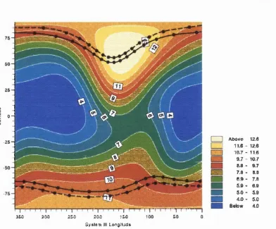
1.2 A shaded contour map of estim ated surface field strength according to the

Oe magnetic field model of Connerney (1991, 1993). The field strength unit

is given in Gauss. P lotted on top of the map are the lo Torus footprint (dots

connected by a solid line) and the footprint of the Last Closed Field Line -

field line 30 R j (dots connected by a dashed line)... 32

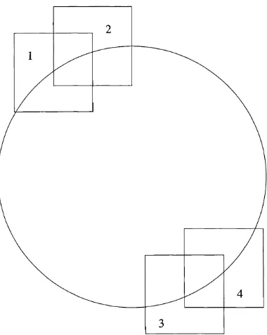
2.1 Positions relative to the center of the planet at which ProtoC am images were

taken in order to achieve complete coverage of the jovian auroral regions. . 51

2.2 A 3.533 /xm mosaic of Jupiter composing of nine separate images. These

were obtained on the 22"^ of April 1993, at the System III CML of 316°. The

most intense emission is shown as orange to yellow, and the least as dark

brown to black. The dashed fines are marking out the lo Torus footprint

(magnetic shell 6 R j) and the footprint of the last closed field fine (magnetic

shell 30 Rj) according to Connerney’s Oe model (1991, 1993). An elliptical

“surface” of Jupiter was drawn around the planet to aid with the alignment

(8)

2.3 A 4,0 fi m mosaic of Jupiter composing of nine separate images. These were obtained on the 23^^^ of April 1993, at the System III CML of 189°. The

most intense emission is shown as orange to yellow, and the least as dark

brown to black. The dashed lines are marking out the lo Torus footprint

(magnetic shell 6 R j) and the footprint of the last closed held line (magnetic

shell 30 Rj) according to Connerney’s Oe model (1991, 1993). An elliptical

“surface” of Jupiter was drawn around the planet to aid with the alignment

of the images... 54

2.4 Diagram showing how the limb-brightening correction was computed for a

point on the disk of the planet. The line of sight ratio is taken to be the

ratio of the perceived gas length, L, to the gas scale height, H . It is assumed

th a t the radius, R , has not changed appreciably going from the surface of

the planet to the outer edge of the gas layer. 0 is the com puted latitude of

the desired point on the planetary disk... 57

2.5 Spectrum of the standard taken at 3.5 f i m ... 61 2.6 Spectrum of standard star taken at 4,0 f i m ... 62

2 . 7 Graphs showing a 3.45 /xm spectrum fitted using a theoretical H3 emission

spectrum broadened by convolving with: (a) Voigt, (b) Gaussian, or (c)

combined Voigt and Gaussian profiles...6 6

2.8 An example of a 2-D spectral image taken at 3.45 f i m wavelength range. The slit was aligned north—south along the rotational axis. The planet

occupies rows 7 (south pole) to 20 (north pole) in the image. A relative

intensity colour scale was used for the im age...6 8

2.9 An example of a 2-D spectral image taken at 3.45 f i m wavelength range. The slit was aligned east—west along the equator. The planet occupies

rows 7 (west) to 20 (east) in the image. A relative intensity colour scale

(9)

2.10 An example of a 2-D spectral image taken at 4.0 jim. wavelength range. The slit was ahgned north—south along the rotational axis. The planet occupies

rows 7 (south pole) to 20 (north pole) in the image. A relative intensity

colour scale was used for the im age... 71

2.11 Two spectra fitted to the same set of data. In the first the continuum

was assumed to be constant at aU wavelength, in the second a polynomial

convolved with an uncorrected spectrum of the standard star was used as

an estim ate of the background level. The fitted tem peratures and column

densities are 1230K and 0.181 mol m “ ^ for the first, 974K and 0.565 mol m “ ^

for the second. The standard deviations are 0.00386 and 0.00344 respectively. 73

2.12 F itted 4.0 /xm spectrum of the northern aurora extracted from the spec

tral image seen in the previous figure. The background used was a scaled

spectrum from the body of the planet...74

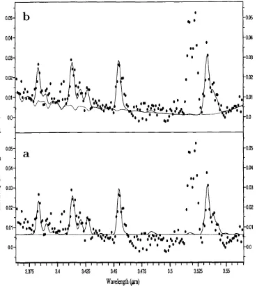
2.13 Graphs of three theoretical spectra fitted to the same d a ta set. Atmospheric

absorption of the 2930.169 cm“ ^ (3.41277 /xm) hne were set at 0, 20% and

40% for graphs shown in a , b and c respectively. The standard deviations

are .03878, .03126 and .05118 for a , b and c respectively... 76

2.14 Contour diagram used to estim ate the uncertainty associated with fitted

tem perature and column density. The contour is drawn at 99% confidence

level for 140 degrees of freedom... 79

2.15 G raph of emissivity per molecule of H3 versus tem perature. The values are

plotted on a logarithmic scale... 81

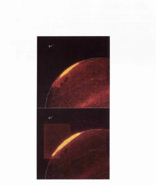
3.1 Images of the H3 north aurora taken at 3.533/xm. Footprints of the IP T

and the LCFL, according to the Oe model, are shown on the images as

dashed hnes. The CML is given in the top left hand corner of each image.

(10)

3.2 Images of the H3 north aurora taken at 3.533)um. Footprints of the IP T

dashed lines. The CML is given in the top left hand corner of each image.

The limb-brightened corrected image is shown at the to p ... 90

3.3 Images of the H3 north aurora taken at 3,533/xm, Footprints of the IP T

3.5 Images of the H3 north aurora taken at 3.533//m, Footprints of the IP T

3.6 Images of the H3 north aurora taken at 3,533/zm, Footprints of the IP T

3.8 Images of the H3 north aurora taken at 3,533//m, Footprints of the IP T

(11)

3.10 Images of the Hg north aurora taken at 3.533/xm. Footprints of the IP T

and the LCFL, according to the Og model, are shown on the images as

The hmb-brightened corrected image is shown at the to p ... 104

(12)

3.16 Images of the H3 north aurora taken at 3.533//m. Footprints of the IP T

3.17 Images of the H3 north aurora taken at 3.533/zm. Footprints of the IP T

The hmb-brightened corrected image is shown at the to p ... I l l

(13)

3.25 Diagram showing how the path length of an emission oval varies depending

on the viewing angle of a distant observer. The column length will be longer

when viewed at A th an when viewed at B and therefore the emission wiU

appear correspondingly brighter... 119

4.1 2-D spectral image of Jupiter. Two white lines running through the middle

of spectral rows show where the edges of the planet is estim ated to be. . . . 127

4.2 Examples of fitted 3.45 /xm spectra from individual rows shown in fig 2.8.

The spectra were taken from rows 20 (c), 14 (b) and 7 (a). The fitted

tem peratures and column densities are 822K and 51.4 x 1 0^^ cm “ ^ for row

20, 755K and 1.44 x 10^^ cm“ ^ for row 14, 786K and 41.6 X 10^^ cm“ ^ for

row 7. The unfitted feature in the spectrum (b) at 3.52 /xm is the “doublet”

referred to by Ballester et al (1994) and in chapter 2 of this w ork...128 4.3 Examples of fitted 4.0 /xm spectra from individual rows shown in fig 2.10.

The spectra were taken from rows 20 (c), 14 (b) and 7 (a). The fitted

tem peratures and column densities were 903K and 43.7 x 10^^ cm ” ^ for row

20, 1019K and 10.47 x 10^^ cm” ^ for row 7. b shows a typical spectrum

(14)

4.4 Mapping of fitted tem peratures onto the surface of Jupiter. Colour shadings

associated with tem perature ranges are given by the legend to the right of

the map. Footprints of the lo Plasm a Torus and the LCFL (Connerney

1991, 1993) are shown by curves connecting the dots on the m ap. Solid

curve for the lo Plasm a torus and dashed one for the LCFL... 133

4.5 Mapping of fitted column densities onto the surface of Jupiter. Colour

shadings associated with column density ranges (units of 1 0^^ cm” ^) are

shown by the legend to the right of the map. Footprints of the lo Plasm a

torus and the LCFL (Connerney 1991,1993) are shown by curves connecting

the dots on the map. Sohd curve for the lo Plasm a torus and dashed one

for the LCFL... 134

4.6 3-D mapping of the computed to tal emission param eter onto the surface

of Jupiter. The emission has been corrected for the limb-brightening effect

and is given in units of 10“ ^ erg s~^ sr“ ^ cm“ ^... 137

4.7 2-D maps of the computed to tal emission. Colour shadings associated

with to tal emission ranges are shown on the right and is given in units

of 10“ ^ erg s~^ sr“ ^ cm~^. The bottom map is a limb-brightening cor

rected version of the top. The auroral boundaries are shown as dashed

lines connecting the dots. The lo torus footprints are shown as solid lines

connecting the dots. Both were computed using Connerney’s Oe magnetic

field model (1991, 1993)... 138

4.8 Shaded contour maps of the computed to tal emission for latitudes between

± 40°. The labelled lines are contours of constant surface magnetic field

strength according to the Oe model. Limb-brightened corrected emission

map is shown in b ...141

4.9 A shaded contour map of the computed to tal emission for latitudes between

± 40°. The labelled lines superimposed on top of the map are contours of constant dip angles of the magnetic field lines according to the Oe model.

(15)

± 40°. The labelled lines superimposed on top of the map are contours of

constant loss cone angles at the magnetically conjugate equatorial point,

according to the offset-tilted dipole model. Limb-brightened corrected emis

sion map is shown in b ... 143

± 40°. The labelled lines are the footprints of m agnetic shells according to

the offset tilted dipole model. Limb-brightened corrected emission is shown

in b ... 144

4.12 G raph of the E(cml) param eter plotted as a function of longitude for the

northern auroral region...146

4.13 G raph of the E(cml) param eter plotted as a function of longitude for the

southern auroral region...147

4.14 Three graphs showing the to tal emission, corrected for the line of sight

effect and normalised to the noon time value. The d a ta were obtained on

the of May 1993 at the CML of 67°. Spectra were taken with the slit

aligned east—west along the equator. The east (rising) limb is to the left

of the graphs. The computed to tal emission is shown in red, line of sight

corrected in green and the blue curve is the to tal emission normalised to the

noon time value and is dimensionless. The black bar to the left of the graph

shows an error value which is typical for aU the computed to tal emission. . 149

the 3^^^ of May 1993 at the CML of 122°. Spectra were taken with the slit

(16)

the 3^^ of May 1993 at the CML of 229°. Spectra were taken with the slit

noon tim e value and is dimensionless. The black bar to the left of the graph

shows an error value which is typical for aU the computed to tal emission. . 151

the 4^^ of May 1993 at the CML of 260°. Spectra were taken with the sht

shows an error value which is typical for all the computed to tal emission. . 152

the 4^^ of May 1993 at the CML of 350°. Spectra were taken with the slit

corrected in green and th e blue curve is the to ta l emission normalised to the

(17)

List o f Tables

4.1 Einstein A%y coefficients for CGS4 3.45 /um fitting... 122

4.2 Einstein k i j coefficients for CGS4 3.45 fi m fitting... 123

4.3 Einstein A i f coefficients for CGS4 4.0 fi m fitting... 124

4.4 Einstein A i j coefficients for CGS4 4.0 fi m fitting... 125

4.5 Results of fitting 3.45 fim spectra with the slit aligned pole to pole. The d a ta were obtained on the 4^^ May 1993 at the CML of 40°. Column densities are given in units of 1 0^^ cm“ ^ and to tal emissions in units of 10~^ erg s“ ^ sr"^ cm~^... 154

4.6 Results of fitting 3.45 fim spectra with the slit aligned pole to pole. The d a ta were obtained on the 5^^ May 1993 at the CML of 47°. Column densities are given in units of 1 0^^ cm“ ^ and to tal emissions in units of 10“ ^ erg s“ ^.sr“ ^ cm“ ^... 155

4.7 Results of fitting 3.45 f i m spectra with the slit ahgned pole to pole. The d a ta were obtained on the 3^^ May 1993 at the CML of 102°. Column densities are given in units of 1 0^^ cm~^ and to tal emissions in units of 10~^ erg s~^.sr” ^ cm“ ^... 156

(18)

4.9 Results of fitting 3.45 fim spectra with the slit aligned pole to pole. The d a ta were obtained on the 3^^ May 1993 at the CML of 180°. Column

densities are given in units of 1 0^^ cm“ ^ and to tal emissions in units of

10~^ erg s~^ sr“ ^ cm“ ^... 158

4.10 Results of fitting 3.45 fi m spectra with the slit aligned pole to pole. The d a ta were obtained on the 3*"^ May 1993 at the CML of 210°. Column

10“ ^ erg s~^ sr~^ cm“ ^... 159

4.11 Results of fitting 3.45 fim spectra with the slit aligned pole to pole. The d a ta were obtained on the 4*^ May 1993 at the CML of 241°. Column

1 0“ ^ erg s~^ sr~^ cm” ^... 160

4.12 Results of fitting 3.45 fi m spectra with the slit aligned pole to pole. The d ata were obtained on the 3^^ May 1993 at the CML of 254°. Column

1 0“ ^ erg s~^ sr~^ cm“ ^... 161

4.13 Results of fitting 3.45 fi m spectra with the slit aligned pole to pole. The d a ta were obtained on the 3’’^ May 1993 at the CML of 324°. Column

1 0“ ^ erg s“ ^ sr“ ^ cm~^... 162

4.14 Results of fitting 3.45 fim spectra with the slit aligned pole to pole. The d ata were obtained on the 4*^^ May 1993 at the CML of 325°. Column

10“ ^ erg s~^ sr“ ^ cm“ ^...163

4.15 Results of fitting 4.0 fi m spectra with the slit aligned pole to pole. The d ata were obtained on the 5*^ May 1993 at the CML of 26°. Column

(19)

4.16 Results of fitting 4.0 fim spectra with the slit aligned pole to pole. The d a ta were obtained on the 5^^ May 1993 at the CML of 92°. Column

densities are given in units of 1 0^^ cm~^ and to tal emissions in units of

10“ ^ erg s~^ sr“ ^ cm~^...164

4.17 Results of fitting 4.0 f im spectra with the sht ahgned pole to pole. The d a ta were obtained on the 3^^ May 1993 at the CML of 160°. Column

10"^ erg s“ ^ sr“ ^ cm“ ^...164

4.18 Results of fitting 4.0 fim. spectra with the sht ahgned pole to pole. The d a ta were obtained on the 3^^^ May 1993 at the CML of 196°. Column

10“ ^ erg s“ ^ sr“ ^ cm~^...165

4.19 Results of fitting 4.0 iim spectra with the sht ahgned pole to pole. The d a ta were obtained on the 5^^ May 1993 at the CML of 2 0 2°. Column

10“ ^ erg s“ ^ sr” ^ cm“ ^...165

4.20 Results of fitting 4.0 //m spectra with the sht ahgned pole to pole. The

d a ta were obtained on the 3^*^ May 1993 at the CML of 278°. Column

10“ ^ erg s“ ^ sr~^ cm“ ^...165

4.21 Results of fitting 4.0 fim spectra with the sht ahgned pole to pole. The d a ta were obtained on the 4*^ May 1993 at the CML of 299°. Column

densities are given in units of 1 0^^ cm~^ and to tal emissions in units of

1 0” ^ erg s“ ^ sr“ ^ cm “ ^...166

4.22 Results of fitting 4.0 fi m spectra with the sht ahgned pole to pole. The d a ta were obtained on the 5^^ May 1993 at the CML of 339°. Column

(20)

4.23 Tables of fitted tem peratures and column densities obtained by combining

rows sampling the regions described... 167

4.24 Table of fitted tem peratures and column densities obtained by combining

rows sampling the regions described... 168

4.25 Results of fitting 3.45 //m spectra with the slit aligned east-w est along the

equator. The d ata were obtained on the 5*^^ May 1993 at the CML of 67°.

Column densities are given in units of 10^^ cm“ ^ and to tal emissions in

units of 10“ ^ erg s“ ^ sr“ ^ cm“ ^... 169

4.26 Results of fitting 3.45 //m spectra with the slit aligned east-w est along the

equator. The d ata were obtained on the 3^"^ May 1993 at the CML of 122°.

units of 10“ ^ erg s~^ sr” ^ cm” ^... 170 4.27 Results of fitting 3.45 ^m spectra with the slit aligned east-w est along the

equator. The d ata were obtained on the 3^^ May 1993 at the CML of 229°.

units of 10“ ^ erg s“ ^ sr~^ cm~^... 171

4.28 Results of fitting 3.45 fi m spectra with the slit aligned east-w est along the equator. The d ata were obtained on the 4*^^ May 1993 at the CML of 260°.

units of 10"^ erg s“ ^ sr“ ^ cm~^... 172

4.29 Results of fitting 3.45 fi m spectra with the slit aligned east-w est along the equator. The d ata were obtained on the 4*^ May 1993 at the CML of 350°.

Column densities are given in units of 10^^ cm"^ and to tal emissions in

units of 10“ ^ erg s” ^ sr“ ^ cm~^... 173

A .l Example of a colour scale defined using the R G B scheme. The colours go

from black through orange to yellow...2 1 0

A.2 Example of file containing coordinates defining features on the surface of

Jupiter. This file defined points on the northern and southern footprint of

(21)

(22)

A cknow ledgem ents

I would like to begin by thanking my supervisors, Steven Miller and Jonath an Tennyson,

who have given me encouragement and support throughout my time with the group. Their

readings and discussions have made my thesis far b etter than I can accomplish alone.

My thanks also to all the people in group C for their help and encouragements, es

pecially Nicholas Achilleos for his advice and discussions. They have given me a b etter

understanding of the concepts and processes involved in the subject.

I would like to express my thanks to Gilda Ballester, Bob Joseph, Tom Geballe,

Jack McConnel and Renée Frangé whose advice on a number of topics have been very

welcomed indeed.

I’m grateful to SER C/PPA RC for a studentship and grants to atten d conferences and

go observing as part of my studies.

For most of the time during my study Tina Rehm gave me her whole support and

encouragement for which I’m forever indebted. I ’m sorry th a t things did not tu rn out the

way she expected.

I ’m enormously grateful to my parents who have supported me both financially and

w ith their encouragements when I most needed them.

Finally, I would like to thank the Linden Gardens Mob and the Clanricarde Trio for

putting up with me when no one else would, M aurette CahiU for p utting a bit of light

chaos into the project and Vito Graffagnino who not only understands the words “dress”

and “sense” in th a t order, but whose inane banter has kept me from going insane aU these

(23)

C h a p te r 1

In trod u ction

1.1 Laboratory M easurem ents o f

In his “Further Experiment on Positive Rays” J. J. Thomson (1912) reported discovering

an ion with a mass to charge ratio of 3:1. After considering other possibilities he concluded

th a t the molecule formed from three hydrogen atoms. But theory at the tim e could

not account for such a system being chemically bound and Thom son was consequently

persuaded th a t the ion was a deuterated hydrogen molecule. The existence of H3 was

only accepted when Hirschfelder (1938) finally showed th a t the molecule was stable and

strongly bound.

Hg is the simplest, stable polyatomic system. Its equilateral triangle configuration at

equihbrium means th a t it does not have a pure rotational spectrum . Theoretical consider

ations also showed th a t Hg does not have any stable excited electronic state (apart from

a triplet state close to its second dissociation lim it). Thus, H ^ spectrum would only be

observed spectroscopically in the infrared (I.R.), through its doubly degenerate 1/2 bending

mode (the z/% symmetric stretch mode is Raman active only).

The search for the infrared spectrum of Hg was initiated by Herzberg in 1967 but

its discovery in 1980 by Oka had to wait for the high sensitivity of laser spectroscopy.

Although many more hnes have since been recorded and assigned, progress has been

(24)

the spectral lines of Hg are spaced unevenly, making it difficult to predict new transitions

from the positions of known lines.

Right from the sta rt, the detection and interpretation of the Eg spectrum was made

possible by basic theoretical calculations, beginning with th e remarkable work of Hirschfelder

(1938). The introduction of computers (Christoffersen et al 1964) into the process was a great step forward. Calculations by Carney and P orter (1974, 1976) resulted in the first

relatively accurate prediction of the ro-vibrational spectrum of the ion. The electronic

surfaces calculated by Meyer, Botschwina and B urton (1986) were used in spectroscopic

calculations to achieve very high accuracy (MiUer and Tennyson 1989, 1988). This led di

rectly to the identification of the molecule outside of the laboratory. The latest theoretical

calculations dem onstrate the remarkable advances made in this field, now showing th a t the

largest error in the calculation of transition frequencies is due to the Born-O ppenheim er

approxim ation (DineUi et al 1994, and review by Tennyson 1995).

In astrophysics Hg has a key role in interstellar chemistry. It is formed through the

ionisation of molecular hydrogen and then the rapid reaction:

H } + H 2 — ^ H + + H (1.1) Normally very reactive the molecule is destroyed in the interstellar medium through

dissociative recombination:

H + + e H^ + H

H + H + H (1.2) and th e reaction:

H } + X H X + + H2 (1.3) which is extremely efficient for chemical species whose proton affinities are greater th an

those of H2 (Flower 1990).

Hg has a m ajor role in the gas phase interstellar chemistry as well as hydrogen plasm a

(Lequeux and Roueff 1991). In the cold, hostile environment of the interstellar medium,

H J acts as a protonating agent, via reaction 1.3, explaining the observed abundances of

(25)

Prior to 1988 attem pts to detect H3 concentrated solely on the interstellar medium,

in particular the Orion and Taurus molecular clouds where H3 is believed to occupy a

key role in the gas chemistry. Because of the low tem perature in the interstellar environ

m ent, efforts were focussed whoUy on searching for the H3 absorption spectrum . To date,

however, no positive identification of the ion has been made (Oka 1981, Geballe and Oka

1989, Black et al 1990).

1 .1 .1 E x t r a - T e r r e s t r ia l D e t e c t io n o f H j

The ionosphere of Jupiter had been considered by numerous workers as a possible source

of the ion (A treya et al 1974, Hunten 1969). A treya and Donahue (1976) proposed a model of the jovian atmosphere where concentrations of H3 reached 1 0^ cm“ ^ in a thin

layer (<50 km) close to the homopause.

The Low Energy Charged Particle experiment on board Voyager did detect an ion

with a mass to charge ration of 3:1 in the jovian magnetosphere (Hamilton et al 1980). These authors suggested th a t the jovian ionosphere could be a significant source of the

H3 molecule. McConnell and Majeed (1987) modelled the jovian ionosphere controlled by

solar EUV and found Hj" concentration as high as 10^ cm“ ^ around 1000 km above the

am m onia cloud tops.

The first remote identification of H3 outside the laboratory was made by D rossart et al

in 1989. They were attem pting to observe the quadrupole spectrum of molecular hydrogen

on Jupiter. These transitions, occurring around 2//m, are intrinsically weak; H2 Einstein

A i f values are typically 10“ ^ s“ ^. However column densities of H2 in Jupiter are about

10^^— 10^^ cm“ ^; large enough to make spectroscopic observations feasible. The attem p t

was successful. But Drossart et al (1989) also found a number of lines which were even more intense than the quadrupole transitions they were looking for. Trafton et al (1989) had earlier reported the same unassigned lines, although at much lower resolution.

The eventual identification of the lines as the overtone {2u2{l = 2) —>■ 0) transitions of H3 owed at least as much to highly accurate quantum calculations (Miller and Ten

(26)

instrum ents in astronomy.

1.2 Jupiter

1 .2 .1 P la n e t a r y S t r u c t u r e

The largest planetary body in the solar system is composed mainly of hydrogen and

helium in solar proportion (H e/H ~0.11). G ravitational soundings, observing the orbits of

Ju p ite r’s moons and spacecraft trajectories have enabled theorist to construct a model of

the planet.

According to Smoluchowski (1976), the center of the planet may be a rocky core of

heavy m aterial about the size of the E arth. Surrounding the core is a m antle of hydrogen

and helium m ixture, which is either solid or liquid at the base and gaseous at the top. The

helium may be distributed to provide the non-homogeneity required in order to account for

the observed gravitational field. Motions of satellites are strongly affected by the density

gradient in the outside few percent of the planet’s radius, consequently the structure in

this region is better known than deeper in.

Heat balance indicates th a t Jupiter is em itting more than twice the energy it receives

from the Sun. This implies a high central tem perature of 20000 K or more and the

planet being nearly aU liquid or fluid. Internal heat tran spo rt is therefore, dom inated by

convection.

High conductivity and low viscosity associated with the metallic interior enables the

operation of a hydromagnetic dynamo to take place. This is driven by planetary rotation

and therm al convection which in turn, generates the huge magnetic field observed around

Jupiter.

1 .2 .2 A t m o s p h e r e

Ju p ite r’s atm osphere is fascinating in term s of visual appearance and dynamics. Conse

quently, a large body of work already exists on the subject. For a comprehensive view of

(27)

Here, we will give a brief summary of the compositions and tem perature profiles of the

atm osphere and ionosphere.

Ju p ite r’s visual appearance is dominated by clouds and their motions. Q uantitative

description is difficult however and their compositions is usually determined through theory

(A treya 1986, Chamberlain and Hunten 1987). The atmosphere is mostly H2 with about

10% He. The visible cloud layer is composed of solid NH3, with additional NH4SH and

H2O layers at pressures of 3 and 5-7 bars respectively. There is evidence for the existence

of CO, PH3, GeH4 and HCN (D rossart et al 1982, Lellouch et al 1984). The colouring

m aterial of the clouds have been much speculated about and ranges from organic m atters

to red phosphorus, but as yet there is still no observational identification of the colourants.

The atmospheric therm al profile can be seen in figure 1.1 (taken from Hunten 1976).

At the 1 bar pressure level the tem perature is 170 K and decreases going up through

the troposphere to a minimum of 100 K at the tropopause (0.1 bar). The tem perature

then increases throughout the stratosphere, leveling out at the stratopause. Tem perature

remains constant in the mesosphere up to the mesopause, conventionally defined as the

base of the thermosphere. From here on the tem perature increases rapidly to 850 K at

pressure of 1 0“ ^ ^bar.

Height measurements of atmospheric structures are made with respect to some arbi

trary level since Jupiter has no surface. The usual practice is to either locate the feature

on a pressure scale or to specify the height with respect to some pressure level such as the

H2O cloud base (5-7 bar), ammonia cloud tops (1 bar), 1 m bar and 1 ^bar.

Results from Pioneer 10 and 11 radio occultation measurements showed th a t th e elec

tro n density profile in Ju p iter’s ionosphere has up to seven peaks. A model by A treya

and Donahue (1976) indicated th a t the ionosphere is dominated by protons. However, in

a thin layer (<50 km) close to the homopause, concentration of the H^ ion can reach up

to 1 0^ cm~^ and become the dominant species.

Kim and Fox (1991) modelling the ionospheric E region, found two strong solar lines

penetrating below the m ethane homopause to ionise the hydrocarbons (mostly C2H2).

(28)

Figure 1.1: Therm al profile of Ju p iter’s atmosphere (taken from H unten 1976). For levels

(29)

located around 320 km above the ammonia cloud tops. H ydrocarbon ions are quickly

converted to more complex species through reactions w ith CH4, C2H2, C2H4 and C2H6.

The ionospheric tem perature of Jupiter is high. Radio occultation d a ta from the Pio

neer 11 encounter indicated a plasma tem perature of 850±100 K. A treya (1986) proposed

particle precipitation and Joule heating as the most likely mechanisms to account for the

heat source. However, both particle precipitation and Joule heating are localised at the

auroral regions. An efficient convection system is therefore needed to distribute the energy

deposited at the aurorae to regions throughout the ionosphere.

The collision of the comet Shoemaker-Levy/9 with Jupiter in the summer of July

1994 presented a unique opportunity to witness an event of unparaUel m agnitude in the

solar system. It prom pted a huge international effort, both to observe and model the

consequences th a t arise when a large comet or asteroid collide with a planetary body. An

enormous am ount of work was carried out to monitor the effects on Jupiter due to the

im pact. In particular, a modelling effort by Abouelainine, Mangeney and D rossart (1995)

dem onstrated th a t horizontal circulation combined with vertical convection can be very

efficient at distributing the energy of the im pact throughout the atm osphere. However, it

is not known whether large scale vertical motions exist in the therm osphere and above.

Nevertheless this gives a hint about the mechanism required for energy deposited in the

auroral region to be transported to lower latitudes in the ionosphere.

1.2.3 Jovian M agn etosp h ere

The first clue to the existence of a magnetic field on Jupiter came with the detection

of low-frequency radio emission by Burke and Franklin (1955). At the tim e Jupiter was

considered to be a giant sphere of gas surrounded only by space. G round-base monitoring

of non-therm al radio emissions yielded basic characteristics of the m agnetic field such as

southw ard polarity, approxim ate tilt angle of the magnetic dipole axis with respect to

the rotational axis and crude estimates for the dipole moment and surface field intensity.

A comprehensive discussion about the observations and interpretations of jovian radio

(30)

The Pioneer encounters in the early 1970’s and the Voyager fly-bys in 1979 added a

wealth of inform ation about the magnetic field and magnetosphere of Jupiter. In p ar

ticular, the spacecraft provided in - s itu measurements of the magnetic field and plasm a environm ent, and maps of the ultraviolet(U.V.) and I.R. emissions associated with mag-

netospheric processes. The discovery of a plasma torus surrounding the planet at about

6 R j revealed a strong electrodynamic interaction between Jupiter and its moon. To (Kupo,

Mekler and E viatar 1976).

Jupiter possesses the largest planetary magnetic moment in the solar system. Its enor

mous magnetosphere extends out to 50-100 jovian radii from the planet. W hen discussing

the jovian magnetosphere, it is custom ary to consider the three following regions.

In n er M a g n eto sp h e re

This region of the jovian magnetosphere begins at the “surface” of Jupiter and extends

out to 6 R j. The magnetic field in this region is predominantly due to currents in the

planetary interior (Acuha et al 1983). The effects of the m agnetotail and the azim uthal current are unim portant. The widely held view is th a t the magnetic field is generated by

a therm al convection-driven dynamo in the electrically conducting region of the planetary

interior. Field variations in m agnitude and direction take place over long tim e scales. The

field is smoothly varying when observed along spacecraft trajectories.

The inner magnetosphere contains a torus of cold plasma between 5.3 R j and 5.6 R j.

The warm torus begins at the orbit of lo ( 6 R j) , extending to 7.5 R j. The lo plasm a

torus is the m ajor source of plasm a for the entire magnetosphere. This is in contrast with

the E arth, which lacks a significant internal plasma source (Strobel 1989).

M id d le M a g n eto sp h e re

The magnetic field in this region is dominated by an equatorial current sheet (magnetodisc)

beginning at the orbit of lo ( 6 R j) and extending to 30-50 R j. The internal magnetic

field can be approxim ated by a dipole plus small contributions from the magnetopause and

(31)

radial components to the nearly dipolar internal field, leading to stretching of field lines

in the radial direction, along the plane of the current sheet. The current sheet is tilted

with respect to the rotational equator resulting in a 1 0 hour periodic “rocking” motion.

The middle magnetospheric region is regarded as a transition stage between the ambient

(alm ost dipolar) internal field and the magnetodisc geometry of the outer magnetosphere.

O u ter M a g n eto sp h e r e

From 30-50 R j to the magnetopause (^^100 R j) the magnetic field is highly distorted

due to the interaction with the solar wind. The field has a large southw ard component

and shows large spatial and tem poral variation as a direct response to the changing wind

pressure. The region also includes the extensive m agnetotail, which harbours charged

particles stream ing away from the planet in the anti-solar direction.

Because of the asymm etry of the outer magnetosphere, discussions always differentiate

between the “sunwards side” and the “magnetic tail.”

The magnetopause on the sunwards side is the region where stream ing particles from

th e solar wind encounter the jovian magnetic field. It is a boundary layer separating the

outside region where the magnetic field is determined by the motions of charged particles,

from the region where the movements of charged particles are restricted by the internal

field. Solar wind particles encountering this boundary are swept around the planet to

eventually precipitate into the atmosphere through open field lines, or to end up in the

planetary bow shock (a region in the solar wind shadow, on the anti-solar side of the

planet).

The jovian m agnetotail contains a large current sheet separating the northern and

southern lobes of the local magnetic field. Across the current sheet the field reverses

direction and field lines tend to he paraUel to the equatorial plane of Jup iter at increasingly

(32)

M a g n e tic F ie ld M o d e l

In term s of observing Ju p iter’s auroral emissions, a magnetic field model of the relevant

region is essential to interpret the data. To this end a number of m agnetic field models

have been proposed, the most notable of which are the O4 model of Acuna and Ness

(1976), the P11(3,2)A model of Smith, Davis and Jones (1976) and m ost recently, the Oe

model by Connerney (1991,1993) which is derived by considering an explicit model of the

magnetodisc.

Ju p ite r’s magnetic field can be represented, to first order, by an offset tilted dipole

model. However, measurements (Connerney et al 1982) indicated th a t contributions from higher order magnetic multipoles are non-neghgible. AU models mentioned above attem p t

to incorporate these higher order components so as to accurately reproduce spacecraft

m easurements. In addition, the models are used to make im portant predictions or to

explain aspects of observations (made either from spacecraft or from ground-based ob

servatories). The derivation of magnetic field models is outside the scope of this work.

Detailed descriptions can be found elsewhere (Acuna and Ness 1976, Smith, Davis and

Jones 1976, A treya et al in Physics of the Jovian M agnetosphere (1981)). The paper by Connerney (1991) gives detailed accounts of the procedure used to derive the Oe model.

A brief description wiU be given of the theory required to reproduce (numericaUy) the Oe

model of Connerney.

ModeUing the inner region of the magnetosphere begins with the assum ption th a t there

are no significant current sources in this region, i.e. current density

J

= V x B « 0. The

field B can then be represented by a sum of scalar potentials

B = - v y = -v(y= r )

(1.4)

where V® and V* represent sources external and internal to the region respectively.

V can be expanded in terms of spherical harmonics (Chapm an and Bartels 1940, Langel

(33)

Here a is the equatorial planetary radius and r is the radial distance. T® and are series representing contributions from external and internal sources respectively. The two

are expressible in term s of Schmidt-normalised associated Legendre functions

Ê {Pni'^0^9) [G:coa(mÿ) + H^sin{m4,)]} (1.6)

771 = 0

{P n {(^o se ) [g^cos{m(i>) + sin{m (j))]} (1.7)

771=0

where 0 and </> are the normal right handed spherical polar angles, 0 (denoting colatitude)

measured from the rotational ajds and 0 increasing in the direction of rotation. System

III longitude is obtained by taking 360 — (j). and are the external and internal Schmidt coefficients respectively.

In practice, given the sparseness of the observations, the series is usually truncated at

some order n = Nmax-, where Nmax is taken to be large enough to accurately represent the measurements but not so large so as to introduce more free param eters than can be

determined by observations. The O4 model of Acuha and Ness (1976) incorporates term s

up to and including n= 3 for the internal coefficients but nothing for the external term s.

The P11(3,2)A model of Smith, Davis and Jones (1976) incorporates term s up to and

including n= 3 for the internal coefficients but also has term s up to an including n = 2 for

the external ones.

The recent Oe model of Connerney (1991, 1993) is an attem p t to make improvements

on the O4 model (Acuna and Ness 1976). It is essentially a partial solution, consisting

of the first three orders of a six-order expansion of the source function. Like the O4

model of Acuna and Ness (1976), the Oe (Connerney 1991, 1993) model only incorporates

internal coefficients for term s up to and including n=3. Unlike the O4 (Acuha and Ness

1976) model however, the Oe model (Connerney 1991, 1993) provides for the possibility

(34)

ë 0

-m ?

m

[ 1 Above 12.0

I I 11.6 * 12.6

10.7 - 11.6 9.7 - 10.7 8.8 - 9.7 7.8 - 8.8 6 . 9 - 7.8 5.9 - 6.9 5.0 - 5.9 4.0 - 5.0 Below 4.0

350 300 250 200 150

System III Longitude

Figure 1.2: A shaded contour map of estimated surface field strength according to the Oe

magnetic field model of Connerney (1991, 1993). The field strength unit is given in Gauss,

Plotted on top of the map are the lo Torus footprint (dots connected by a solid line) and

the footprint of the Last Closed Field Line - field line 30 Rj (dots connected by a dashed

(35)

A shaded isocontour map of to tal surface field intensity as predicted by the Oe (Con

nerney 1991, 1993) model can be seen in figure 1.2. This shows th a t the m agnetic field

is highly asymmetric. The maximum surface field strength is about 14 G in the north

and about 10 G in the south. In addition the high field strength is concentrated in a

smaller region in the north th an in the south. The model is also used to map footprints of

constant magnetic shells on to the surface of the planet. This is invaluable in predicting

ionospheric and atmospheric signatures of processes taking place in the magnetosphere.

Im portant examples are the precipitation into the atmosphere of charged particles from

the lo plasm a torus, and observations of emissions from the foot of the lo flux tube.

The term Last Closed Field Line (LCFL) is used here to denote the field line crossing

the equator at a distance of 30 R j from the centre of the planet. This has been widely

employed to mean the boundary between closed field lines and field lines connecting to the

interplanetary medium, its footprints on the surface of the planet indicating the auroral

boundaries beyond which particle precipitation is thought to occur on open field fines. It

should be noted th a t this boundary is highly variable, indeed U.V. observations (Frangé,

private communication) show th a t north and south auroral emissions may be conjugated

indicating closed field fines in th a t region. Only emissions at the poles may, therefore, be

attrib u ted with confidence to open field fines.

1.2.4 T h e Influence o f lo

lo F lu x T ube

Strong control of the decametric emissions by the Galilean satellite, lo, was well established

before the planetary missions, through the monitoring of jovian radio emissions (Bigg 1964,

Desch et al 1975, C arr and Desch 1976, Goldstein and E viatar 1979, Leblanc 1981)). Explanations of this phenomenon were put forward by Piddington and Drake (1968)

and Goldreich and Lynden-Bell (1969). The widely accepted hypothesis, based on a strong

electrodymanic interaction between lo and the corotating jovian ionosphere, is given the

term “unipolar inductor.” Ions and electrons are accelerated by this unipolar generator to

(36)

is an emission hot spot whose area is restricted by the flux tube intercepting lo. Such a

spot has been observed by A treya et al (1977) and, recently, by Connerney e t al (1993). Extensive observations and discussions have been made on the natu re of the lo flux

tube, whose scope is beyond th a t of this work. Reviews in P h y sic s o f the J o v ia n M a g n e  tosphere (A. J. Dessler, ed., 1983) and T im e-V a ria b le P h e n o m e n a in the J o v ia n S y s te m

(Belton, West and Rahe, 1989) give more comprehensive discussions.

lo P la sm a T orus

Brown (1974) reported optical observations of neutral sodium connected with lo ju st before

the Pioneer 10 encounter. The subsequent discovery of a plasm a torus at the orbit of lo

was made by Kupo, Mekler and Eviatar (1976) when they observed optical emissions due

to S'*" from a region ju st inside Jo’s orbit. This was interpreted by Brown as coming from

a dense ring of cold plasma.

Because of its highly volcanic nature lo injects a great number of particles into the

magnetosphere. Ablation of m aterial from the surface of lo due to im pacting particles also

makes a substantial contribution.

According to Schardt and Goertz (1983) it is thought th a t plasm a from the various

sources (ionosphere, solar wind, etc.) initially diffuses outwards to the m agnetotail under

centrifugal and plasm a pressure. In this region plasm a is accelerated to high energies

(MeV) and then diffuses back in towards the planet, due to pressure gradient instabihties,

to eventually end up in the vicinity of lo. It is here th a t charged particles are lost to

the magnetosphere due to various mechanisms, i.e. atmospheric precipitation, charge-

exchange, etc.

The lo plasm a torus is made up of two parts (Belcher 1983). The cold inner torus

inside of 5.6 R j, is confined to the centrifugal equator and has a scale height of ~0 . 2 R j

(Kupo et al 1976). The warm outer torus extends from the orbit of lo (5.9 R j) to about 7.5 Rj and has a scale height of about 1.0 R j (Broadfoot et al 1979). This discovery

prom pted a substantial shift of focus away from the solar wind, to the lo torus as the

(37)

1.2.5 Ionosp h eric E m issions

Emissions from the jovian auroral regions at UV and IR wavelengths have been observed

bo th by spacecraft and ground-based observatories. In addition, low level emission, term ed

“electroglow,” was observed by Voyager to em anate from all areas of the planet. The

emissions arise from particle precipitation and Joule heating which, in tu rn , are linked

to physical processes taking place in the magnetosphere. To interpret the emissions it is

necessary to have some idea of these magnetospheric processes and their consequences for

the atmosphere.

M a g n e to sp h e ric P r o c esse s

According to Bryant (1993) a charged particle from the solar wind encountering Ju p ite r’s

m agnetic field will either precipitate into the atmosphere or be deflected from its path. The

outcome is dependent on the particle’s momentum per unit charge (known as magnetic

rigidity), P , and the strength of Ju p iter’s magnetic field, B , where P is defined by:

I."

Z e is the particle’s charge, p is the particle’s momentum, E and Eq are its kinetic and rest energy in electron-volts, and c is the speed of light in a vacuum. P is in term s of volts.

Reaching Ju p ite r’s surface is possible only if P is > > / B x dl, where d \ is an element of trajectory. The integral / B x dl represents the impulse experienced by the particle on

crossing the magnetic field lines. Therefore, for a given energy, a particle is much more

likely to reach Ju p ite r’s atmosphere if its approach is close to the polar regions, w ith its

velocity is nearly parallel to the magnetic field, than if it approaches the planet near the

equatorial plane, where its velocity is nearly perpendicular to the field lines.

For solar wind particles, precipitation will occur over the whole of the polar regions

giving rise to diffuse auroral emissions.

For a charged particle injected inside Ju p iter’s magnetosphere, escape is difficult. The

particle may either precipitate into the planetary atm osphere or become trap ped in the