Bedding control on landslides: a methodological approach for computer-aided mapping analysis

(1)

www.nat-hazards-earth-syst-sci.net/11/1395/2011/ doi:10.5194/nhess-11-1395-2011

and Earth

System Sciences

Bedding control on landslides: a methodological approach for

computer-aided mapping analysis

G. Grelle, P. Revellino, A. Donnarumma, and F. M. Guadagno

Dipartimento di Studi Geologici e Ambientali, Universit`a del Sannio, via dei Mulini, 59/A, 82100, Benevento, Italy Received: 3 September 2010 – Revised: 20 January 2011 – Accepted: 10 April 2011 – Published: 16 May 2011

Abstract. Litho-structural control on the spatial and tem-poral evolution of landslides is one of the major typical aspects on slopes constituted of structurally complex se-quences. Mainly focused on instabilities of the earth flow type, a semi-quantitative analysis has been developed with the purpose of identifying and characterizing litho-structural control exerted by bedding on slopes and its effects on lands-liding. In quantitative terms, a technique for azimuth data in-terpolation, Non-continuous Azimuth Distribution Method-ological Approach (NADIA), is presented by means of a GIS software application. In addition, processed by NADIA, two indexes have been determined: (i)1, aimed at defining the relationship between the orientation of geological bedding planes and slope aspect, and (ii)C, which recognizes local-ized slope sectors in which the stony component of struc-turally complex formations is abundant and therefore oper-ates an evolutive control of landslide masses. Furthermore, some Litho-Structural Models (LSMs) of slopes are pro-posed aiming at characterizing recurrent forms of structural control in the source, channel and deposition areas of grav-itational movements. In order to elaborate evolutive models controlling landslide scenarios, LSMs were qualitatively re-lated and compared with1andCquantitative indexes. The methodological procedure has been applied to a lithostruc-turally complex area of Southern Italy where data about az-imuth measurements and landslide mapping were known. It was found that the proposed methodology enables the recog-nition of typical control conditions on landslides in relation to the LSMs. Different control patterns on landslide shape and on style and distribution of the activity resulted for each LSM. This provides the possibility for first-order identifica-tion to be made of the spatial evoluidentifica-tion of landslide bodies.

Correspondence to: F. M. Guadagno

(guadagno@unisannio.it)

1 Introduction

Geological and structural settings of slopes are the main pre-disposing factors controlling mass movement development (Fookes and Wilson, 1966; Zaruba and Mencl, 1969; Varnes, 1978). Bedding of lithologically or structurally complex se-quences (sensu Esu, 1977; Vv. Aa.; 1985), stratigraphic or tectonic contacts between rocks with different geomechani-cal properties, and zones of intense fracturing linked to the presence of axes of folds and faults are all geological con-ditions at the basis of structural control (e.g. Guzzetti et al., 1996; Irfan, 1998; Scheidegger, 1998; Cruden, 2000; Martino et al., 2004; Margielewski, 2006; Prager et al., 2009). The definition of these elements at different scales plays a fundamental role in understanding the landsliding mechanism. Where landslide processes are the main mod-elling agents, bedding planes of layered formations can control both the landslide mechanism and the activity, in terms of style and distribution (cf. WP/WLI, 1993; Cruden and Varnes, 1996). Therefore, the definition of the litho-structural setting is a basic aspect in landslide susceptibil-ity assessment, as its spatial prediction implies careful eval-uation of the geo-structural conditions in areas where both first-time and reactivated events can develop.

The analysis of the relationship between bedding plain at-titude and topography can be a key procedure in identify-ing and comprehendidentify-ing the structural control on slope and landslide evolution. Moreover, the abundance, the frequency and/or distribution and the geomechanical characteristics of the stony component within the sequences, in comparison to the more clayey part, may produce a different morpho-evolutive behaviour of slopes.

(2)

For nearly two decades, the necessity to perform geo-structural analyses on a large scale has induced some authors to introduce computer-aided methods to the spatial distribu-tion of azimuth data. Some interpoladistribu-tion techniques aimed at obtaining spatially distributed fields of the orientation of ge-ologic fabrics (in this case bedding-slope relationship) have been presented in scientific literature. One of these is the TOBIA-index (TOpographic/Bedding plane Intersection An-gle), proposed by Meentemeyer and Moody (2000). Even though this index provides the conformity between slope and bedding planes by means of the computation and the digital mapping of their intersection angle, model outputs are not unique due to the continuous representation. By using the direction cosines (de Kemp, 1998; G¨unther, 2003) for de-composing irregularly distributed attitude measurements, the interpolation of azimuth data avoids the occurrence of nu-merical gaps in crossing over Cartesian quadrant boundaries, instead. Nevertheless, the direction cosines method interpo-lates azimuth measurements in a continuous manner. There-fore, it does not provide for discontinuity thresholds due to sudden and wide azimuth variations in adjacent points. For example, interpolation between two azimuth values at inter-vals of about 180◦is portrayed rather as an idealized continu-ous semicone-shaped surface than as a fold, which represents the most frequent natural condition.

This paper describes and presents a new computer-aided methodology, NADIA (Non-continuous Azimuth DIstribu-tion methodological Approach) aimed at producing a both continuous and discontinuous distribution of azimuth data in relation to typical and recurrent geological settings. A set of computational procedures has been developed as well, aimed at slope characterising and modelling in terms of structural control. By means of discrete data processing of geometrical slope parameters and orientation of geological features (bed-ding planes), simple determinations of slope sectors where structural control plays a key role on the development and evolution of landslide phenomena have been computed.

Furthermore, this study identifies and proposes some Litho-Structural Models (LSMs) of slopes, aiming at recog-nizing recurrent and specific litho-structural settings which may control landslide evolution. The study area corre-sponds to an inland sector of the Southern Italian Apennine, mainly characterized by instabilities of the earth flow type (Guadagno et al., 2008).

2 A very complex geological environment

The lithological and structural complexity of an area is often one of the main factors characterizing landslide-prone con-ditions. In mountainous areas, such as the Italian Apennines, the influence of tectonic phases on lithologically complex se-quences has produced peculiar settings that represent predis-posing causes controlling the spatial evolution of landslides. This background is representative of the morphological

evo-5 km

135 1005

m a.s.l.

4584703.22N 4584703.22N

2501367.32E

4556416.57N 4556416.57N

2526247.54E

Tammaro River Fortore River

Apennine Watershed

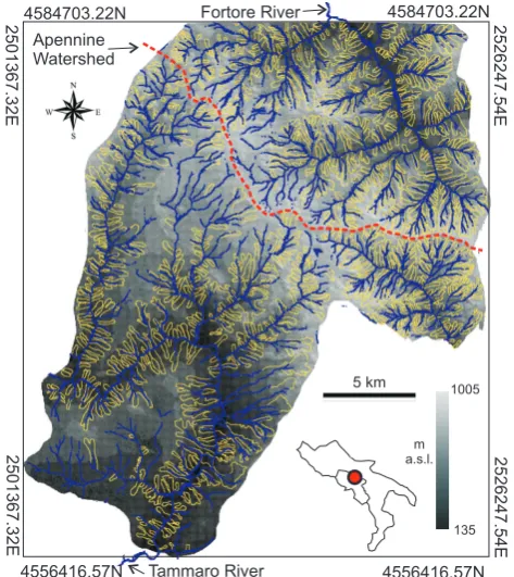
Fig. 1. Location map and DEM of the study area. Landslide distri-bution (data from Guadagno et al., 2006) is shown in yellow.

lution of slopes in the Benevento province (Southern Italy), where slow-moving landslides are particularly widespread in some areas, giving to the region a distinctive feature. Surveys and multitemporal analyses have shown that most of these in-stabilities are structurally-controlled or directly connected to the local geological setting both in the source area and along the channel or the accumulation area (Revellino et al., 2010). The pilot area (about 440 km2), belongs to a sector of this province. It includes parts of two catchment basins, selected in order to cover a variety of geological conditions (Fig. 1): (1) the northeastern sector of the Fortore River basin, and (2) the southwestern part of the Tammaro River basin. Con-cerning the morphological setting, the first one is charac-terised by a dendritic erosion pattern and the second one by a more complex trend of the drainage pattern, prevalently im-posed on tectonic lineaments related to transtensive tectonic phases. Moreover, the data on landslide types and pattern (Guadagno et al., 2006) show that slope instabilities are are-ally distributed (Fig. 1) and they mainly consist of earth flows with a restricted number of translational, rotational and pound slides. Sometimes translational, rotational or com-pound movements are only limited to the source areas.

(3)

or more specifically, by similar lithotypes according to their lithology and engineering-geological/geomechanical features. With regards to the area investigated in this paper, two of the five groups of sequences were found; each of them includes more than one lithotechnical unit. They are:

(1) Dominantly pelitic sequences with a high-degree of

tectonization. These include (i) clayey-marly sequences, and

(ii) fully clayey sequences. Rocks are prevalently incompe-tent, from mildly to intensely folded; normally clays appear scaly.

(2) Stony and complex successions with a high-degree

of tectonization. These consist of (i) calcareous-clayey

se-quences organized in well stratified strata and banks, and (ii) arenaceous-clayey and arenaceous-conglomeratic sequences consisting of mainly arenaceous and conglomeratic banks and subordinate thin layers of marls, clays and conglomer-ates. Both sequences are intensely jointed and folded.

The structural setting of the area is rather complex due to thrust-belt structures of carbonate and silico-calcareoclastic terrains and wedge top/piggy-back basin successions. The regional structure of the Chain is the result of some main tectonic phases (D’Argenio et al., 1973; Patacca and Scan-done, 2001): (i) older compressive phases, which produced multiple trusts associated to anticlines and synclines com-plex systems, and (ii) more recent extensional phases with prevailing normal and strike-slip faulting and persistent and diffused jointing.

During compressive phases, flysch sequences generally showed a differentiated response to deformation. The rela-tive abundance of stony layers favoured a prevalently frag-ile behaviour resulting in jointing at different scales. As the clayey component increased, deformation occurred without loss of continuity at basin scale. Therefore, the stony layers are characterized by a dense fissure pattern and, where the clay and shale component abounds, this latter has resulted in parasitic minor folding and scaly structures.

3 Methods of analysis and processing

Two spatial distribution indexes,1andC, have been com-puted to define the bedding-slope relationship and recognize the stony component of the sequences, which operates an evolutive control of landslide masses, respectively. Since the orientation of a geologic fabric is well defined by the dip and the dip direction,1andCcalculation requires the estimation of the following variables: (i) slope aspect or exposure (ψS;

0–360◦); (ii) azimuth of bedding plane (ψL; 0–360◦); (iii)

slope angle (α; 0–90◦); (iv) dip angle (β; 0–90◦).

It should be noted that the spatial distribution of azimuth, which represents a point data, becomes a major aspect in calculating1andC. This distribution should suit the spa-tial variability of azimuth measurements, which is typically observed in geologically complex environments. In most cases, the geological complexity and poor and limited

out-crops make the full reconstruction of a clear structural frame-work very difficult. This aspect motivated the development of a continuous/discontinuous (non-continuous) distribution method of azimuth data, NADIA (Non-continuous Azimuth DIstribution methodological Approach).

3.1 Azimuth data interpolation (NADIA)

Angular data processing through GIS tools cannot be under-taken directly using standard techniques for the spatial distri-bution of data. This is due to the fact that a circular domain is associated to these variables. Therefore, interpolation tech-niques of the “one-way” type cannot be used. In addition, in most cases, actual settings due to tectonic effects show a continuous spatial trend for narrow angle ranges only (layer distortion); in contrast, the spatial trend acquires a discontin-uous character for wide angular ranges.

With the aim of avoiding the described approxima-tion, a methodological procedure, NADIA, has been imple-mented, which joins matrix operations (GRID) of angular and trigonometric data in Boolean algebra to standard tech-niques of spatial interpolation. Data processing and the spa-tial distribution of variables have been performed by means of ArcView GIS Platform (ESRI, 1999) implemented with Spatial Analyst and Grid tool extensions and 3-D Analyst modules. Moreover, all angles in degrees (azimuth and dip) have been converted in radian.

NADIA is founded on the periodicity and, therefore, on the continuity shown by the sine and cosine trigonometric functions in the circular domain. Angle values turned into sine and cosine can be interpolated in a continuous and two-way manner. For this purpose and in contrast to stochas-tic techniques, the application of IDW (Inverse Distance Weighting) deterministic interpolation methodology (Davis, 1986) guarantees that the spatial distribution of the trigono-metric variables is defined in the finite domain [−1 to 1]. Moreover, IDW applied to trigonometric values permits the following advantages (Fig. 2): (i) if interpolation occurs in a narrow range of values, the trend of interpolated data fits the sine and cosine function trend (conditions A and B in Fig. 2); (ii) if interpolation occurs in long angular arcs, the trend of interpolated data intersects the sine and cosine func-tion (condifunc-tion C in Fig. 2). This implies that spatially distributed trigonometric data is continuous for narrow an-gle ranges and discontinuous for wide angular ranges (right side of Fig. 2). Additionally, as two angular values are respectively associated to sine and cosine in different Carte-sian quadrants of the 0–2π domain, their independent in-terpolation enables the production of unique outputs, mak-ing it possible for azimuth values to fall into the right quad-rant. Once the quadrant is identified, the final value results from the arithmetic mean of angles produced by the inverse trigonometric function sine and cosine.

Therefore, in order to spatially distributeψL, the first step

(4)

-1 -0.5 0 0.5 1

0

0 0

45 45

90 90

135 135

180 180

225 225

270 270

315 315

360 360

0 20 40 60 80 100

A

C

B

A B

T

rigonometric values

Degree

Degree (°)

Distance Invsin

Invsin

Invcos

Invcos Mean

Mean

Mean Invcos

Discontinue

Continue

Prevalent continue

sine cosine

90 180 270 360

Fig. 2. Linear interpolation of sine and cosine (left side) and their angular distribution by applying IDW (right side; Davis, 1986) in different simulated conditions: (A) short arcs within the quadrant; (B) short arcs across quadrant boundary; (C) long arcs across quadrant boundary.

-1.00

a)

b)

1.00

0.00

Fig. 3. Spatial distribution of sinψL(a) and cosψL(b) by IDW technique. Azimuth point measurements are shown by blue spots.

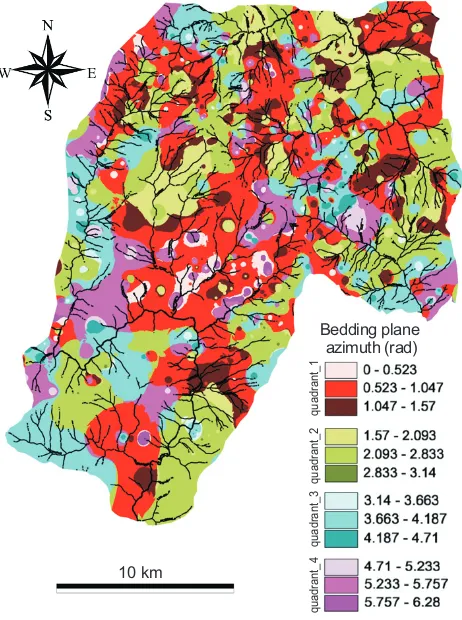
means of the IDW technique (Fig. 3). For the present study, we used 633 azimuth measurements collected from field sur-veys and from 1:25 000 to 1:100 000 scale official geologi-cal maps (Servizio Geologico d’Italia, 1971; Pescatore et al., 2008; ISPRA, 2011).

(5)

quadrant_1

quadrant_2

quadrant_3

quadrant_4

Bedding plane azimuth (rad)

10 km

Fig. 4. Spatial distribution of bedding plane azimuths (ψL)by

NA-DIA.

[quadrant 1] = (([sinψL]>0) and ([cosψL]>0) · ([sinψL]

.ASin + [cosψL] .ACos)/2;

[quadrant 2] = (([sinψL]>0) and ([cosψL]<0)

·(π– [sinψL] .ASin + [cosψL] .ACos)/2;

[quadrant 3] = (([sinψL]<0) and ([cosψL]<0)

·(π– [sinψL] .ASin + 2π– ([cosψL] .ACos)/2;

[quadrant 4] = (([sinψL]<0) and ([cosψL]>0)

· (2π+([sinψL] .ASin +2π – ([cosψL] .ACos)/2;

conse-quently:

[ψL] =

4 X

n=1

[quadrant n]

where .ASin and .ACos correspond to sin−1 and cos−1, re-spectively and all the map calculator functions are reported in italic.

Figure 5 shows some examples of linear interpolation be-tween two points which are at a distance of 100 units of mea-surement by using the methodology described above. As it is possible to observe, the azimuth distribution is contin-uous for angle ranges not exceeding 40◦–60◦; in contrast,

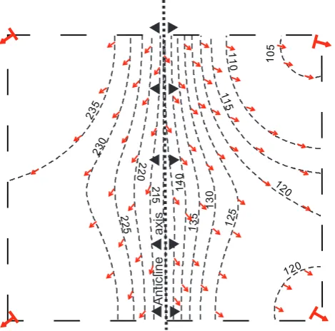
wider ranges result in a discontinuous distribution, as oc-curs when folds and angular unconformity are present. How-ever, it should be noted that the linear interpolation process of sine and cosine variables produces different distributions regardless of the bound value of the considered ranges. In particular, (i) in discontinuous distributions, few interme-diate anomalous angular values can be exhibited (Fig. 5c), (ii) a discontinuous pattern is shown by narrow angle ranges across adjacent quadrants (Fig. 5d). In Fig. 6 an example is given of the spatial representation of the azimuth distribution of a hypothetical anticline fold.

3.2 The1-index

The bedding-slope relationship can be locally defined by the 1-index, which can be expressed by the following relation-ship:

1=0.5−(|ψS−ψL|/π ) (1)

having the physical condition that|_ψ_S−ψL|< π.

The1-index, which assumes values in the finite domain [−0.5 to 0.5], describes the structural setting of three types of slopes (Fig. 7) as categorized by Powell (1875): (a)

cat-aclinal slope, if bedding planes dip in the same direction as

the slope; (b) orthoclinal slope, if the azimuth of the dip di-rection is orthogonal to the azimuth of the slope didi-rection, and (c) anaclinal slope, if bedding planes dip in the direction opposite to the slope. Furthermore, the continuous character of1also defines intermediate slope orientations,

plagiocli-nal slope (Callaway, 1879), which is useful for describing the

remaining slopes oblique to the strike of the bedding. The spatial distribution ofψs(Fig. 8) is derived from

high-resolution Digital Elevation Model (DEM)-data (5 m); ψL,

on the other hand, can only be obtained by field measure-ments. This contains the limitation that measurements are restricted where bedding layers outcrop; therefore, ψL

as-sumes a “point-to-point” character. In addition, both for its physical (angle) and geological (azimuth) nature, the spatial interpolation ofψLmust take into account the following

con-ditions: (i) existence limited to the finite domain [0; 2π], (ii) behaviour depending on the direction (zeroing to the north), and (iii) discontinuous distribution due to the presence, for example, of folds or angular unconformities.

As stated above, the 1-index (Eq. 1) is the result of a matrix operation aimed at defining the orientation of geologic fabrics in relation to the slope aspect. In order to guarantee that the function conforms to the directional requirement or it is always valid in the condition|ψS−ψL|<

πsg the following methodological process has been adopted:

[Map1] = ([ψs] – [ψL]) .Abs;

(6)

0 45 90 135 180 225 270 315

0 10 20 30 40

0 45 90 135 180 225 270 315

0 10 20 30 40

0 45 90 135 180 225 270 315

0 5 10 15 20 25 0 45 90 135 180 225 270 315

0 5 10 15 20 25

0 45 90 135 180 225 270 315

0 5 10 15 20 25 0 45 90 135 180 225 270 315

0 5 10 15 20 25

0 45 90 135 180 225 270 315

0 20 40 60

0 45 90 135 180 225 270 315

0 20 40 60

a)

d) c)

b)

Fig. 5. Linear interpolation between two azimuth values which are at a distance of 100 unities of measurement: (a) continuous distribution, (b) discontinuous distribution, (c) non-uniform discontinuous distribution, and (d) non-uniform continuous distribution.

12 5 1 3 0 23 0 13 5 1 4 0 2 2 5 2 2 0 2 1 5 1 2₀ 23 5 1 1 5 1 1

0 10

5

120

Anticline axis

Fig. 6. Spatially-distributed estimates of an anticline with axis strike oriented north-south. For distribution of sine and cosine, the IDW technique is applied with a power of four.

[Map3] = not ([Map1]< π )·[2π- Map1]; and consequently,

[1] =0.5−(([Map1] + [Map2])/2π )

Figure 9 shows the1distribution in the study area, where chromatic variations refer to± 20◦ range around the pure orientation of cataclinal slopes, anaclinal slopes and ortho-clinal slopes as conventionally categorized by Cruden and

yL yL yL yS yS yS a yL

yS b

a yL yS b a yL yS b D D D = 0.5 = 0

= /2p

=p = 0.0 = -0.5

-a)

b)

c)

Slope Bedding plane

Fig. 7. Bedding-slope relationships defined by1for: (a) cataclinal slope, (b) orthoclinal slope, and (c) anaclinal slope.

(7)

Slope aspect (rad)

10 km

Fig. 8. Slope aspect (ψS)derived from high resolution DEM from

a 1:5000 scale topographic map (5 m).

relationship between slope angle and slope area for anaclinal and cataclinal slopes shows similar patterns with maximum values of approximately 11◦(Fig. 9c).

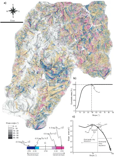
3.3 The structural controlC-index

The stony component within structurally complex formations is often one of the key factors linked to the structural control of landslide bodies. In order to recognise this effect in cata-clinal and anacata-clinal slopes only, the following control index (C) has been defined (Fig. 10a):

C=1tag|α−λ| =0.5−(|ψS−ψL|/π )tag|α−λ| (2)

whereλis a variable depending on the areal distribution ofα in the study area. In particular it is expressed as:

λ=αmax∗−π/4 (3)

whereαmax∗defines the maximum attributed value ofα. As

shown in Fig. 10b, this value is associated with the point that exhibits a sudden and significant change of inclination in the cumulative spatial distribution ofαu In this study,αmax∗

refers to 99 % of the area and corresponds to an angle of 38◦. With regards to the structural control of rocky layers on the evolution of landslides, this control can be recognized by means of specific slope angles connected to the slope classes previously described. Therefore, two finite intervals in the

existence domain ofC have been fixed in relation to speci-fied slope angles. In particular, these conditions are identi-fied by the bi-logarithmic distribution curve of slope angles (Fig. 10c). This distribution shows a quick decrement after reaching the peak value (αpeak)at an angle of 10◦, which can

be compared to the residual shear strength of some typical clays of the area (Grelle and Guadagno, 2010). The bisec-tor of the angle obtained by the intersection of the linear part extension and of the tangent to the peak intercepts the dis-tribution curve in the value namedα*. This latter then aims at identifying the lower threshold defining slope angles influ-enced by the outcrop of stony sequences. In other words, it is assumed that slopes having a slope angle higher thanα* cor-respond to sectors where stony layers are outcropping. For the study area,α* has been found to be equal to 17◦. In par-ticular, it is possible to highlight that, in similar slope areas characterized byαpeak close to 10◦,α* falls into the 10–20◦

range, where the log-diagram has a higher resolution.

4 Litho-Structural Models

Because of the litho-structural features investigated, 1and C quantitative indexes were qualitatively related and com-pared with some simple Litho-Structural Models (LSMs) of the slope. LSMs aim at depicting and schematizing the most recurring litho-structural settings of entire slopes or of slope sectors in the study area in order to elaborate evolutive mod-els controlling landslide scenarios. Correlation between1 andC indexes and LSMs is justified by the fact that, even though areally distributed, these indexes include information regarding the slope attitude (internal geometry). LSMs not only consider the relationship slope/bedding (in particular cataclinal and anaclinal slopes) by means of1but also the presence, the relative abundance and the position (top or bot-tom) of stony layers within sequences by usingC.

In the LSMs, the various sequences do not take into con-sideration the depositional relationship among the different lithological units and the nature of their contacts (sedimen-tary or tectonic). Consequently, three main types of tectonic-stratigraphical sequences can be defined within the LSMs: (i) clayey sequence dominant at the top (TC), (ii) clayey sequence dominant at the bottom (BC), and iii) indistinct clayey sequence (IC). TC and BC sequences relate to the field defined in Fig. 10c. The following most frequent LSMs will be proposed and discussed in the next Paragraphs: (1) LSMs related to cataclinal slopes; (2) LSMs related to ana-clinal slopes; (3) LSMs related to IC; (4) LSMs related to complex settings.

(8)

Slope area Landslide area

Landslide area/Slope area

0

0.30

0.31

0.32 0.33

0.34

0.35

0.37 0.36 5 10 15 20 25 30

D

Area (Km

)

2

-0.50-0.40-0.30 -0.20-0.10 0.000.100.200.300.400.50 Pure anaclinal

slope Pure orthoclinal

slope _{Pure cataclinal}

slope

b)

0 1 2 3 4 5

0 10 20 30 40 50 60 70 80 90 + 20° around the pure

anaclinal slope (D = -0.5)

+ 20° around the pure

cataclinal slope (D = 0.5)

Slope angle (°)

Area (Km

)

2

c)

10 km

a)

D

-0.5 - -0.389

0.5 - 0.389 -0.389 - -0.278

0.389 - 0.278 -0.167 - -0.056

0.167 - 0.056 -0.056 - 0.056 -0.278 - -0.167

0.278 - 0.167

Fig. 9. (a) Grid map of1-index; (b) Spatial distribution of1related to the total slope area and the landslide area; (c) Slope angle versus slope area for anaclinal and cataclinal slopes

4.1 LSMs related to cataclinal slopes

Cataclinal slopes are usually well-known as the most landslide-prone environments. Due to the fact that for this slope type, dip angles may represent the predisposing key factor, LSMs were developed taking into account additional slope categorizations as suggested by Cruden and Hu (1996). Therefore, cataclinal slopes were further divided based on the geometric relationship between the dip of the bedding planes and the slope angle into: (i) overdip slopes, which are steeper than the dip of the bedding plane, (ii) underdip

slopes, which are less steep than the dip of the bedding plane,

and (iii) dip slopes, which follow the bedding plane. Overdip slopes (α > β)with a TC sequence represent one of the most frequent conditions of structural control in the area (Fig. 11a). In this case, the rocky or rocky-clayey mem-ber at the bottom induces a better exposition of the clayey member at the top against actions concurring with landslid-ing. This setting also creates a different morphology

be-tween the landslide source area set upslope and the chan-nel at middleslope, the latter being more steep. This form also influences landslide mobility since a larger amount of potential energy is given to the masses, resulting in a more rapid disposal of landslide debris downslope. Usually, the retrogressive expansion of landslide source areas takes place rapidly. In contrast, overdip slopes with a BC sequence (Fig. 11b) show a strong structural control in the landslide source area, where the main scarp is steep and irregular. Here, rock slides of prismatic blocks frequently occur, feed-ing the clayey visco-plastic mass movement downslope. Ret-rogressive evolution of the landslide body is slow and differ-entiated as well as being influenced by the jointing state of the stony component.

(9)

0 20 40 60 80 100

0 10 20 30 40 50 60 70 80 90

Cumulate area (%)

a

max* a)

b)

c)

1 10 100

Slope area (m

)

2

a_peak

a*

Dominantly clay

sequence _Dominantly stony sequence bisector

line

102 103 104 105 106 107 108

-0.5 tagIa l*_-I -0.5 tagIa_max*-lI

0.5 tagIamax*-lI

0.5 tagIa l*_- I

0.00

-0.50 0.50

Slope angle (°)

-0.22 0.22

Slope (°)

5km

C

Cataclinal slope Anaclinal slope

Fig. 10. (a) Spatial distribution of the structural control index (C)related to slope angle and landslide distribution (in yellow); (b) and (c) distribution curves for defining parameters related to Eqs. (2) and (3) and toCfield action. In the study area:αmax* =α(99%)= 38◦,αpeak=

10◦andα* = 17◦.

a TC–BC-TC multilayered condition is displayed in Fig. 12b, where the spatial distribution ofChighlights how the prevail-ing rocky layers influence the evolution of a landslide system characterized by multiple and superimposed source areas.

The formα∼β generally defines the pure dip slope ori-entation (Fig. 11d). These slopes approach a monoclinal set-ting with slope angles near the residual friction angle of the clayey component. This structural setting, which cannot be

(10)

Fig. 11. Basic recurrent LSMs in TC (clayey sequence prevailing at the top) and BC (clayey sequence prevailing at the bottom) sequences: TC (a) and BC (b) related to overdip slopes (α > β); BC (c) linked to underdip slopes (α < β); pure dip slopes (d) withα∼β; TC (e) and BC (f) related to anaclinal slopes. Legend: (1) landslide body; (2) clayey level; (3) stony level.

500m 500m

C

0.00

-0.50 -0.22 0.22 0.50

Cataclinal slope Anaclinal slope

Stony increase Stony increase

a) b)

Flow direction

Structural control boundary

4572005.46N 4572942.82N

2514014.32E 2515067.87E

2514907.24E

2515961.44E

4571510.56N

4572323.92N

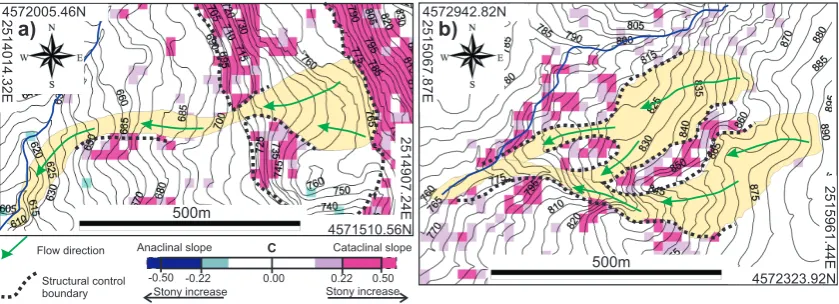
Fig. 12. Structural control on landslides (in yellow) linked to: (a) BC sequence and underdip slopes (α < β); (b) TC-BC-TC multilayered sequence and overdip slopes (α > β).C-index scale is also shown.

4.2 LSMs related to anaclinal slopes

The structural setting is characterised by bedding dipping into the slope. In this case, sliding surfaces, since they do not correspond to bedding planes, are more irregular and mainly influenced by the fracturing condition of the masses.

Control induced by a TC sequence (Fig. 11e) can be gen-erally compared to that of the same sequence in cataclinal slopes, as stated above. Only some minor differences can be identified principally resulting in a greater influence on the evolutive development of the landslide process. Typi-cal examples of these LSMs are the St. Andrea and Serra

delle Forche landslides (Fig. 13). Both of them show a clear

slope change between the clayey top and the rocky-clayey

bottom. In the case of the St. Andrea landslide, the slid-ing material suffers a partial constraint and it divides around more competent strata and comes together again further to the northwest (Fig. 13a). Instead, a total control can be ob-served for the Serra delle Forche landslide. In this case, the presence of a bedding plane of a stony sequence controls the shape, orientation and evolution at the source area, inducing a widening towards the north and the northeast. From the source, the mass movement forms a cross channel-like fea-ture (Fig. 13b). The similar structural control of the two land-slide bodies may suggest that the Serra delle Forche event is a more mature form in comparison to the other.

(11)

Flow direction

Structural control boundary

1000m

C

0.00

-0.50 -0.22 0.22 0.50 Cataclinal slope Anaclinal slope

Stony increase Stony increase 500m

a)

b) 4568708.29N

4561931.55N

2514165.64E

4568016.78N

2515222.07E

2510564.76E

4559918.02N

2513236.96E

Fig. 13. Structural control on landslides (in yellow) related to TC sequences and anaclinal slopes: (a) landslide map, frontal photograph and schematic representation of the Sant’Andrea landslide; (b) landslide map, photograph and schematic representation of the Serra delle Forche landslide (Photos courtesy of Guido Lupo).C-index scale is also shown.

1000m

Flow direction

Structural control boundary Fault

C

0.00

Stony increase Stony increase 4567461.87N

2513946.14E

251663.57E

4565670.02N

(12)

Fig. 15. Rock blocks floating on a landslide body downslope (Photo courtesy of Guido Lupo).

Anaclinal slope

Orthoclinal slope

Cataclinal slope

D D

5Km

D

Coalescent landslide basin: a) boundary of the basin b) coalescent landslides

a)

b)

Fig. 16. Coalescent landslides in a sector of the Fortore River re-lated to1distribution.

irregular source areas. This may be principally due to the frequency and persistence of jointing in the stony member (Fig. 14). For large and deep-seated landslides, it is frequent to find prismatic rock blocks of various dimensions floating on the clay mass in visco-plastic movement (Fig. 15).

Finally, the fan-shape morphology of the accumulation zone seems to be a recurrent and a common condition both in TC and BC sequences when the structural conditioning causes a narrowing of the channel.

4.3 LSMs related to IC sequences

In the presence of IC sequences, it seems that the influence of the bedding plane orientation on landslide evolution is quite poor. Landslide patterns ascribed to coalescent earth-flow systems (sensu Revellino et al., 2010), that is, systems formed by several generations of landslides that mobilise and interact, can be found where slopes are constituted of more or less homogeneous clay formations. These groups of land-slides can be considered as an entity from a morphological point of view as they occur within a sub-catchment. Values as high as 75 % or more of the Landslide Index (LI), calcu-lated as the percentage of area affected by landslide events per 1 km2 grid, are associated to these sectors (Guadagno et al., 2006). Additionally, systems like these but more evolved originate morphological shapes with associated den-dritic drainage patterns.

Figure 16 shows the1distribution, and coalescent land-slide systems as well, in a sector of the study area where these geo-morphological conditions can be recognised. The lack or shortage of the stony component within the sequence makes theC-index useless to be used.

4.4 LSMs related to complex settings

In some cases, spatial distributions of 1 and C point out complex conditions of structural control, which should be explained by means of a combination of the LSMs described above.

(13)

Fold axis

1 Km 500 metres

Outcrop of stony layers

C

0.00

Anaclinal slope

Orthoclinal slope Cataclinal slope 4565005.79

4563113.37

2515546.36

2513358.93

D

Fig. 17. Landslide occupying the nucleus of a syncline: (a)1distribution in the source area and channel of the landslide; (b) schematic cross-section (1–2); (c)Cdistribution and evidence of the stony layers.

Dip slope base

Transcurrent fault

Normal fault

San Giorgio la Molara village

C

0.00

a

b b

Dip Slope

Fig. 18. Structural control operated by dip slopes and fault slope se-ries and schematic cross-section of the geo-structural setting. Land-slide are shown in yellow.C-index scale is also shown.

An “in series” structural control is recognized in Fig. 18. TheC index identifies a series of sandstone dip slopes or-thogonal to the main slope and locally translated by normal or strike-slip faults. The sandstone banks provide a structural control on the development of landslides, which occur within the clayey member.

5 Discussion and conclusion

The proposed methodological procedure permits the obtain-ment of quantitative information regarding the control of litho-structural settings on slope evolution and landslide de-velopment. The bedding plain distribution is the main re-quirement for a mapping analysis. However, this distribu-tion cannot be performed by the usual GIS interpoladistribu-tion tech-niques. This is due to both the geometrical nature of azimuth data and, more in general, to the real complexity of the geo-logical setting.

Unlike continue azimuth interpolation techniques (e.g. de Kemp, 1998; Meentemeyer and Moody, 2000; G¨unther, 2003), NADIA operates both in continue and in discontinue modality in order to perform azimuth distribution and con-stitutes the base for mapping quantitative indexes related to structural control.

Specifically, NADIA considers both the directional nature of the angular datum and the possibility to implement dis-continuous spatial distributions in the case of wide angular ranges, due to faults, folds and angular unconformities. Nev-ertheless, since discontinuities are only recognized by wide azimuth variations between adjoining point measurements without taking into account the bedding dip, this method may approach the actual setting in all but a few cases. For exam-ple, this might occur if folds with a high inclination of the axis (>70–80◦) are present. In this case, changes in azimuth values actually happen in a continuous manner. If this is the case, fictitious strike/dip measurements could be added be-tween real points with the aim of reducing the azimuth gap and therefore enabling NADIA to work continuously.

(14)

to both the total slope surface and the landslide surface (Fig. 9b). This character suggests that bedding planes may not produce a predominant influence on landslide suscepti-bility in areas which are highly tectonized. This outcome is also supported by the similar mapping distribution of catacli-nal and anaclicatacli-nal slopes in relation to slope angle (Fig. 9c), where it seems that the common peaks can be related to the residual shear strength of the clayey component (Grelle and Guadagno, 2010). This aspect confers to this index a me-chanical “threshold” condition, governing the mobility of landslide masses even where the stony component is dom-inant.

Structural control on landslide evolution and shape, and therefore on style and distribution of the activity, can be ob-served from the comparison between theCdistribution and landslide distribution. A decisive control role results when rocky layers within the sequences prevail whatever the orien-tation of bedding planes (cataclinal or anaclinal slope) may be.

Moreover, schematisation of some recurrent settings in re-lation to landslide occurrence and behaviour by means of the LSMs points out that tectonic structures in TC and BC sequences, which are locally characterized by a significant stony component, promote structural control conditions in different sectors of landslide bodies. In particular, depend-ing on their abundance and orientation, stony levels may in-fluence: (i) the retrogressive expansion of the source area, where, in addition, secondary falls, topples, translational slides or lateral spreads of rock blocks might occur; (ii) the channel zone, causing narrowing, flow deviation or jump as in the St. Andrea event (Fig. 13a); and iii) the accumulation modality and, therefore, the toe morphology. Landslides in IC sequences, where the stony component is poor or sparsely distributed, seem to not suffer the influence of both tectonic structures and bedding plane attitudes. These environments show a widespread landsliding, where mass movements rep-resent the main morpho-evolutive factor characterised by co-alescent landslide systems of entire basins.

This study contributes to highlighting that the structural control on landslides is a typical and characteristic factor in structurally complex formations. It influences susceptibil-ity, magnitude and activity (in particular the distribution of the activity) of landslides. As a consequence, the approach introduced, which also permits detecting some control con-ditions in relation to behavioural base models (LSMs), may be used for spatial analyses of landslides and to indicate the most likely future behaviour in similar environmental con-texts. In particular, it also provides the possibility for first-order identification to be made of the spatial evolution of landslide bodies. Such identifications may become a useful tool for improved landslide susceptibility studies and hazard analysis in geologically complex areas.

Finally, future enhancements of NADIA are being devel-oped directed toward improved deterministic susceptibility analyses in different geological environments.

Acknowledgements. The author would like to thank Rinaldo

Genevois, Domenico Calcaterra, and an anonymous reviewer for useful and valuable comments. This work has been funded by the Benevento Province and the Department of Geological and Environmental Studies of the University of Sannio in Benevento (Italy)

Edited by: O. Katz

Reviewed by: R. Genevois and D. Calcaterra

References

Callaway, C.: On plagioclinal mountains, Geol. Mag., 15, 216–221, 1879.

Cruden, D. M.: Some Forms of Mountain Peaks in the Canadian Rockies Controlled by their Rock Structure, Quartern. Int., 68– 71, 59-65, 2000.

Cruden, D. M. and Hu, X. Q.: Hazardous modes of rock slope movement in the Canadian Rockies, Environ. Eng. Geosci., 2, 507–516, 1996.

Cruden, D. M., and Varnes, D. J.: Landslide Types and Processes, in: Landslides: Investigation and Mitigation, edited by: Turner A.R. e Shuster R. L. Sp. Rep., 247, Transportation Research Board, National Research Council, National Academy Press, Washington D.C., 36–72, 1996.

D’Argenio, B., Pescatore, T. S., and Scandone, P.: Schema ge-ologico dell’Appennino Meridionale, Acc. Naz. Lincei, Quad. 183, 49–72, 1973.

de Kemp, E. A.: Three-dimensional projection of curvilinear geo-logical features through direction cosine interpolation of struc-tural field observations, Comput. Geosci., 24, 3, 269–284, 1998. Davis, J. C.: Statistics and data analysis in geology: New York,

John Wiley and Sons, (2nd ed.), 646 pp., 1986.

Environmental Systems Research Institute (ESRI): Arcview GIS 3.2., Environmental Systems Research Institute Inc., Redlands, California, USA, 1999.

Esu, F.: Behaviour of slopes in structurally complex formations, Proc. Int. Sym. on The Geotechnics of Structurally Complex For-mations, Capri, 2, 292–304, 1977.

Fookes, P. G. and Wilson, D. D.: The geometry of discontinuities and slope failures in Siwalik Clay, Geotechnique, 16, 4, 305–320, 1966.

Grelle, G. and Guadagno, F. M.: Shear mechanisms and viscoplas-tic effects during impulsive shearing, G´eotechnique, 60, 2, 91– 103, 2010.

Guadagno, F. M., Revellino, P., Grelle, G., and Lupo, G.: Structurally-controlled earth flows in Campania Apennines (Southern Italy), in: Landslides and Engineered Slopes, From the Past to the Future, edited by: Chen, Z., Zhang, J., Li, Z., Wu, F., Ho, K., Proc. of the 10th Int. Sym. on Landslides and Engi-neered Slopes, 30 June – 4 July 2008, Xi’an, China, Taylor and Francis Group, London, I, 365–371, , ISBN 978-0-415-41196-72008, 2008

Guadagno, F. M., Focareta, M., Revellino, P., Bencardino, M., Grelle, G., Lupo, G., and Rivellini, G.: La carta delle frane della provincia di Benevento, Sannio University Press., Pubb. n. 2906/2006 of CNR-GNDCI, 2006.

(15)

En-viron. Eng. Geosci., 2, 4, 531–555, 1996.

G¨unther, A.: SLOPEMAP: programs for automated mapping of geometrical and kinematical properties of hard rock hill slopes, Comput. Geosci., 29, 865–875, 2003.

Irfan, T. Y.: Structurally controlled landslides in saprolitic soils in Hong Kong, Geotechnical and Geological Engineering, 14, 215– 238, 1998.

ISPRA: Foglio n◦419 “San Giorgio la Molara”. Nuova Carta Ge-ologica d’Italia - scala 1:50.000. Progetto CAR.G. – Finanzia-mento Regione 1996, in press, 2011.

Margielewski, W.: Structural control and types of movements of rock mass in anisotropic rocks: Case studies in the Polish Flysch Carpathians, Geomorphology, 77, 47–68, 2006.

Martino, S., Moscatelli, M., and Scarascia Mugnozza, G.: Qua-ternary mass movements controlled by a structurally complex setting in the Central Apennines (Italy), Eng. Geol., 72, 33–55, 2004.

Meentemeyer, R. and Moody, A. W.: Automated mapping of con-formity between topographic and geological surfaces, Comput. Geosci., 26, 815–829, 2000.

Patacca, E. and Scandone, P.: Late thrust propagation and sedimen-tary response in the thrust belt-foredeep system in the Southern Apennines (Pliocene-Pleistocene), in: Anatomy of an Orogen: The Apennines and Adjacent Mediterranean Basins, edited by: Vai, G. B. and Martini, I. P., Kluwer Academic Publ., 401–440, 2001.

Pescatore, T., Di Nocera, S., Matano, F., Pinto, F., Quarantiello, R., Amore, O., Boiano, U., Civile, D., Fiorillo, L., and Martino, C.: Geologia del settore centrale dei Monti del Sannio: nuovi dati stratigrafici e strutturali, Mem. Descr. Carta Geol. D’It., 77–94, 2008.

Powell, J. W.: Exploration of the Colorado River of the West and its Tributaries. Government Printing Office, Washington, DC, 291 pp., 1875.

Prager, C., Zangerl, C., and Nagler, T.: Geological controls on slope deformations in the Koefels Rockslide area (Tyrol, Austria), Aus-trian Journal of Earth Sciences, 102, 2, 4–19, 2009.

Revellino, P., Grelle, G., Donnarumma, A., and Guadagno, F. M.: Structurally-controlled earth flows of the Benevento Province (Southern Italy), Bull. Eng. Geol. Env., 69, 3, 487–500, doi:10.1007/s10064-010-0288-9, 2010.

Scheidegger, A. E.: Tectonic predesign of mass movements, with examples from the Chinese Himalaya, Geomorphology, 26, 37– 46, 1998.

Servizio Geologico d’Italia: Carta geologica d’Italia alla scala 1:100.000. Foglio n. 173 Benevento”, 1971.

Varnes, D. J.: Slope movement, types and processes, in: Landslides analysis and control, edited by: Schuster, R. L. and Krizek, R. J., Transportation Research Board, National Academy of Sciences, Washington, D.C., Special Report 176, 11–33, 1978.

Vv. Aa.: Geotechnical Engineering in Italy, An overview, Published on the occasion of the ISSMFE Golden Jubilee, Roma, A. G. I.-Associazione Geotecnica Italiana, 414 pp., 1985.

WP/WLI: A Suggested Method for Describing the Activity of a Landslide, Bullettin of the I.A.E.G., 47, 53–57, 1993.