Asymptotic Analysis for Blocking Probabilities of Optical Buffer with General Packet-Length Distributions

Published online January 08, 2015 (http://www.sciencepublishinggroup.com/j/ajam) doi: 10.11648/j.ajam.s.2014020601.11

ISSN: 2330-0043 (Print); ISSN: 2330-006X (Online)

Asymptotic analysis for blocking probabilities of optical

buffer with general packet-length distributions

Yasuji Murakami

The department of Telecommunications and Computer Networks, Osaka Electro-Communication University, Osaka, Japan

Email address:

[email protected]

To cite this article:

Yasuji Murakami. Asymptotic Analysis for Blocking Probabilities of Optical Buffer with General Packet-Length Distributions. American Journal of Applied Mathematics. Special Issue: Switched Dynamics with Its Applications. Vol. 2, No. 6-1, 2014, pp. 1-10.

doi: 10.11648/j.ajam.s.2014020601.11

Abstract:

Asynchronous optical packet switching seems to be suitable as a transport technology for the next-generation Internet due to the variable lengths of IP packets. Optical buffers in the output port are an integral part for solving contention by exploiting the time domain. Fiber delay lines (FDLs) are a well-known technique for achieving optical buffers. This work aims to give a highly accurate approximation of the blocking probabilities of the optical buffers for a generally distributed packet length even when the offered load is extremely low. Such a tool is needed for investigating and designing realistic optical packet switches, which will be used for low-offered-load and low-packet-loss optical IP networks. We use the asymptotic expansion for the decay rate, resulting in a highly accurate approximation. By using the fourth order approximation of the decay rate, an accuracy within 10 % was obtained for both the exponential and uniform distribution cases of an offered load greater than 0.3. The approximations established in this work can be applied to investigate multiclass optical buffers for priority queueing.

Keywords:

Asynchronous Optical Switching, Optical Buffers, Blocking Probabilities, General Packet-Length Distributions

1. Introduction

The ultimate capacity of the Internet may be constrained by energy density limitations and heat dissipation considerations rather than by the bandwidth of the physical components [1]. Recent studies show that optical packet switches do not appear to offer significant throughput improvements or energy savings compared to electronic packet switches [2]. However, the studies also show that optical switch fabrics generally become more energy efficient as the data rate increases [2]. We believe that development of the optical components could lead to a breakthrough in the optical packet switches, and use of all-optical packet switches, in which optical packets are buffered and routed in optical form, will solve the present Internet problems. Asynchronous optical packet switching appears to be suitable as a transport technology for the next-generation Internet due to the variable lengths of IP packets.

In optical packet switches, optical buffers in the output port are an integral part for solving contention by exploiting the time domain. Fiber delay lines (FDLs) are a well-known technique for achieving optical buffers because random access

memory (RAM) is not achievable with current optical technologies. However, optical buffers behave differently from electronic RAM. FDLs can only delay the packets for multiples of a discrete amount of time, called time granularity; the maximum delay is bounded and a packet will be discarded if the maximum delay is not sufficient to avoid contention.

buffers, a numerical algorithm for general cases [8], and a heuristic approach, allowing for simple performance analysis [10], have been provided. However, numerical results only for exponentially distributed packet length were shown.

In our recent work [9], we established a close-form approximate expression for the blocking probabilities and the average delays of the optical buffer, where general packet-length distributions can be applied. For both the uniform and deterministic distributions, the accuracy was high enough in an offered load of greater than 0.7, but decreased when the offered load decreased.

In ITU-T Y.1541 [11], the objective of the end-to-end IP packet loss ratio (IPLR) is recommended to be less than 10-3. Assuming that optical packets pass through a maximum of 100 switches for end-to-end network transmission, the IPLR required for one packet switch is less than 10-5. Packet loss cannot be avoided for the finite FDL optical buffer, and it seems that an IPLR of less than 10-5 is quite difficult to achieve, except in a low offered load.

Our main purpose in this work is to give a highly accurate approximation in closed-form expressions for a generally distributed packet length, even when the offered load is extremely low. Such a tool is needed for investigating and designing realistic optical packet switches, which will be applied for ultra-high-capacity optical IP networks with low offered load and low packet loss. In other words, the present approximation aims at providing an engineering tool for real optical IP network design.

The probability P

(

x>w

)

≡W

( )

x that an arriving customer has the waiting time

w

less than

x

can be approximated to

be the exponential form

( )

x

A x Ce

W =1− −η , where _η is a decay rate and C is a constant. In this work, we use the

asymptotic expansion for the decay rate, and can then obtain a highly accurate approximation even when the offered load is extremely low.

Section 2 briefly reviews the theorems on which our analysis is based [6, 9]. In Section 3, we introduce an asymptotic analysis for the decay rate of the tail probabilities in an infinite optical buffer. The fourth order approximation of the blocking probabilities is given for the generally distributed packet length. In Section 4, we show numerical results and compare them with computer simulation results and exact calculations. Finally, Section 5 concludes this paper.

・

・

・

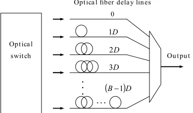
0

Opt ica l

swit ch

D

1

D

2

D

3

･･･

(

B−1

)

D

Opt ica l fiber dela y lin es

Ou t pu t

Fig. 1. Basic structure of optical buffer with fiber delay lines.

void per iod

4

t

3

t t₂ t1

τ

w

iD bu sy per iod n on -fir st a r r iva l pa cket

fir st a r r iva l pa cket

Fig. 2. An example of optical packet flow from optical buffer

2. Optical Buffer Model and Theorems

Our approximation for blocking probabilities is based on the theorems derived by Liu et al. [6] and Murakami [9], so we first briefly review these theorems and notations.

2.1. Model

The basic structure of optical buffers, composed of FDLs, is shown in Fig. 1. Arrived packets can be delayed for a discrete time of

( )

i−1D,1≤i≤B, where D is the time granularity of FDLs and B is the buffer length, to avoid contention at the single output. The maximum delay is T=

(

B−1

)

D; packets with a delay time longer than Tare discarded. All packets are served under the first-come first-served (FCFS) discipline in the optical buffer.

When a newly arrived packet has to wait for at least

w

units of time to be served, the packet is treated as follows. 1)If

( )

i−1D≤w<iD, the packet is switched to the

( )

i+1th

FDL, and a void period

τ

is attached to the head of the packet, where

w iD−

=

τ , iD

D w ₌

   

, (1)

and _{ }x means the smallest integer greater than

x

. 2)If T=

(

B−1

)

D<w, the packet is discarded.

In the case of an FCFS system with Poisson arrivals, the waiting time (that a fictitious packet, which arrived at an arbitrary point of time, has to wait) has the same statistics as the actual waiting time (that each packet spent in the system). Then, we deal with the distribution function of the “virtual” waiting time

x

in stead of the actual waiting time. If a packet arrives, it would have to wait for a duration

x

to get service. The service times of buffered packets are prolonged by a void period

τ

, which introduces excess load compared to the real load. When the buffer is empty and the destination output is free, the packets are transmitted immediately and no void period is attached. The term “PACKET” is defined to indicate the effective service time. There are two kinds of PACKETs;

first-arrival packets, which have no void period and where service times are the real packet lengths, and non-first-arrival packets, which arrive when the buffer is not empty and whose service times are prolonged by the void periods.

right. The output packet at

t

₁ belongs to first-arrival packets and has no void period. The third packet from the head required waiting time

w

to be served when it arrived at the buffer, and the void period

τ

, given by (1), was attached to its head. The buffer becomes empty when the fourth packet flows from the output end at

t

₂. The busy period which consists of the four packets on the right side of the figure, therefore becomes the time from

t

₁ to

t

₂ . At

t

₃ , a

first-arrival packet newly arrives and a new busy period starts.

2.2. Theorems in Infinite Optical Buffer Theorems in Infinite Optical Buffer

We first describe the case of the infinite buffer, i.e., B→∞, where no packet is lost. The following notations are used for the system.

λ Poisson arrival rate

0

s real packet length

( )

x

g₀ probability density function (pdf) of packet length

0

s

( )

x

G₀ cumulative distribution function (CDF) of packet

length

s

₀

0

s

mean value of

s

₀, so ₌∞

_∫

( )

0 0

0 xg xdx

s

ρ offered load, i.e.,

ρ

=

λ

s

₀

( )

x

l pdf of void period

τ

υ

s

service time of non-first-arrival packets, i.e.,

τ

υ =s0+

s

( )

x

g pdf of the service time

s

_υ, so

( )

( ) ( )

_∫

∞

(

) ( )

∞ −

− ≡

⊗

=g x l x g x yl y dy

x

g 0 0 , (2)

where

⊗

shows convolution integral

υ

s

mean value of

s

_υ, so

( )

2 0 0 0

D s s dx x xg

s =

∫

= + = +

∞

τ

υ (3)

( )

x

v steady state pdf of virtual waiting time

x

of

PACKET

( )

x

V steady state CDF of virtual waiting time

x

of

PACKET

Q steady probability of system being empty

eq

ρ equivalent load of PACKET, i.e.,

ρ

eq=1−Q

The following equations were obtained for steady-state system conditions [6].

The equivalent load is given by

ρ ρ ρ

0

2 1

s D

eq

− =

. (4)

When the system is in a stable condition, i.e., ρ_eq<1, the

Laplace transformation of v

( )

x is given by

( )

( )

_{( )}

] 1 [

] 1 [

* * 0 *

θ λ θ

θ λ

θ

g g Q v

− −

−

= , (5)

where *

( )

θ 0

g and _g*

( )

θ _{are the Laplace transformations of}

( )

x

g₀ and g

( )

x , respectively. Equation (5) corresponds to the Pollaczek-Khinchin transform equation in the M/G/1 system [12]. If the denominator will be some rational function of

θ

, finding a particular factored form is desirable.

2.3. Theorems in Finite Optical Buffer

In the finite buffer, if the packet requires a virtual waiting time

x

longer than the maximum allowable delay T=₍B−1₎D,

the packet is discarded. There are three types of PACKETs: 1)first-arrival packets, x=0 and are admitted past the

buffer

2)non-first-arrival packets and admitted packets, 0<x≤T 3)non-first-arrival packets and discarded packets, T <x. The notations used to describe the finite buffer system follow.

T

w

mean packet delay of admitted packets without a void period, which is the average of delays of both type 1) and 2) PACKETs

B

P

packet blocking probability

When ρeq<1, the mean packet delay is given by ( )

( ) ( )     

− + −

=

_∫

T V

Q D dx T V

x V T w

T

T 1

2

0

, (6)

where the third term on the right-hand side is caused by the void periods of the admitted PACKETs, i.e., type 2) PACKETs, whose service times are prolonged.

When ρeq<1, the packet blocking probability is given by

(

)

[

( )

]

( )

[

VT

]

T V PB

− ′ −

− ′ − =

1 1

1 1

ρ ρ

, (7)

where the quasi-load ρ′was introduced [9] as

     

+ = ≡ ′

0

2 1

s D

s ρ

λ

ρ υ , (8)

and all the variables are associated with the infinite buffer system.

3. Our Asymptotic Analysis

solving the inverse Laplace transformations analytically is not easy except for specific functions. The probability

(

x w

)

W

( )

x

P > ≡ , that an arriving customer has the virtual waiting time

w

less than

x

, can be approximated as the exponential function

( )

x

A x Ce

W =1− −η , (9) where η is the decay rate and

C

the proportional constant [13-15]. Equation (9) holds for heavy traffic, i.e., traffic load

ρ

nears 1, and suitably large

x

in the M/G/1 system. If

( )

x W

( )

x

W ≅ A (10)

and we use

( )

0 =1−C=1−ρ

W_A , (11)

we can obtain parameters such as

ρ

=

C

and

η

=

ρ

w. (12)

In our recent work [9], furthermore, we approximated the inverse Laplace transformation of *

( )

_θ

v given by (5) as

( )

(

)

   

   

+ ′ − − −

=

υ

ρ ρ

s x C x

V

g

eq 2

1 1 2 exp

1 , (13)

where 2

g

C is the variance of the service time of the non-first-arrival packets, which is normalized by the square of the mean service time

s

_υ; that is,

(

2 2

)

2

2

υ υ υ s s

s

C_g = − . (14)

By the approximation of (13), we could obtain numerical solutions with high accuracy for the blocking probabilities and the average delays when the offered load was greater than 0.7.

3.1. Asymptotic Expansion for Decay Rate

η

The method of heavy-traffic asymptotic analysis in solving the inverse Laplace transformation for the probability function, such as _v*

( )

θ _{of (5), has been already studied in [13, 14]. The}

decay rate

η

was expanded by a power series of

(

1_−ρ

)

, and each coefficient of

(

_−ρ

)

n

1

(

n=0,1,2,⋯

)

was calculated step

by step. The first-order approximation in the expansion by

(

1−ρ

)

is sufficient for heavy-traffic cases of

α

→

1

limit.

When

ρ

is low, i.e.,

(

1−_ρ

)

is large enough, however, the

higher-order terms are needed to obtain highly-accurate calculations. If the denominator of (5) can be factorized by

θ

, the decay rate

η

is given by a negative root of denominator = 0. Then, we start to solve the negative root of

( )

[

1₋ *

]

₌0

−λ θ

θ g by asymptotically expanding

( )

[

1₋ *₋

]

₌0

−

−η λ g η in powers of

(

1−ρ

)

. The Laplace transformation *

( )

_θ

g of the pdf for the service time of the non-first-arrival packets can be expanded

by

( )

− =∞

∫

( )

0 *

dx x g e g µ ηx

⋯

⋯+ +

+ +

+

= n n

n M M

M

η η

η

! !

2 ! 1

1 1 2 2 _{, (15)}

where M_n is the

n

th moment of g

( )

x , defined by

( )

∫

∞

≡ 0

dx x g x

M n

n . (16)

Equation (15) is called the moment-generating function of

( )

x

g . For example, the first moment is the mean service time of the non-first-arrival packets, such as

2

0 1

D

s

s

M

=

_υ

=

+

, (17)

and the second moment is given by

(

2

)

2

2 s 1 Cg

M = _υ + . (18)

Inserting (15)~(17) into −

η

−

λ

[

1− *

( )

−

η

]

=0

g , we can

obtain

(

)



  

 

+ + + + + =

′

− +

⋯ ⋯ n n

n M M

M

η η

η λ ρ

! 1 !

3 ! 2

1 2 3 2 1

(

)



  

 

+ +

+ + +

′

= +

⋯ ⋯ n n

s n

M s

M s

M _{η η η}

ρ

υ υ

υ 3! 1!

! 2

1 2

3 2

, (19)

where we use ρ′=λs_υ. Equation (19) indicates that the

asymptotic decay rate is expressed in powers of

(

1−ρ′

)

instead of

(

1−ρ

)

.

For expanding (19), we set

(

)

⋯

⋯+ ₊ +

+ +

≡ n+ n

s n

M s

M s

M

A

η

η

η

υ υ

υ 3! 1!

! 2

1 2

3 2

+

+

+

+

=

n

n

b

b

b

1

η

2

η

2

⋯

η

, (20)

where

(

n

)

sυ

M

b n

n

! 1

1

+

= +

. (21)

Assuming the conditions of

η

,A<1, we can expand (19) in powers of A and obtain the equation in powers of

η

, i.e.,

⋯

+

−

+

−

=

′

−

2 3 4

1

ρ

A

A

A

A

(

) (

3

)

3 1 2 1 3 2 2 1 2

1

η

b b

η

b 2bb b

η

b + − + − +

=

(

)

[

4

]

4

( )

5

1 2 2 1 2 2 3 1

4 2bb b 3b b b

η

O

η

b − + + − +

where we show up to the fourth term of

η

.

In (22), 1−_ρ′is given by the polynomial of

η

. According

to the reverse transformation formula [16],

η

is also expressed by the polynomial of

1

−

ρ

′

, i.e.,

(

)

(

)

(

)

3

3 2 2

11 ρ 1 ρ 1 ρ

η=a − ′ +a − ′ +a − ′

(

)

4

(

(

)

5

)

41−ρ′ + 1−ρ′

+a O , (23)

where each coefficient is given by

(

)

υ υ s C M s b a g 1 1 2 2 1 2 2 1 1 + = =

= _{, (24)}

3 1 2 1 2 2 b b b

a =− − , (25)

(

) (

)

5 1 3 1 2 1 3 1 2 2 1 2 3 2 2 b b b b b b b b

a = − − − + (26)

(

)(

)

[

3 1 2 1 3 2 1 2 1 7 1

4 5 2

1 b b b b b b b b

a = − − +

(

) (

₂

)

3

]

1 2 4 1 2 2 1 3 1 2 2 4 2

1 b b 2bb 3b b b 5b b

b − − + − − −

− (27)

Hereafter, we call the asymptotic series in which greater-than-

n

th terms are truncated, as in (23), the

n

th order approximation. Note that the first order approximation of (23) is used in (13)

3.2. Asymptotic Expansion for Proportional Constant

C

Table 1. Moments for service time distributions for non-first arrival packets

moments Exponential Deterministic Uniform

1 M

2 1+D

2 1+D

2 1+D

2 M 3 2 2 D D+ + 3 1 2 D D+ + 3 3 4 2 D D+ + 3 M 4 3 6 3 2 D D D+ +

+

(

)

D D

4 1

1+ 4−

4 2 2 3 2 D D D+ + + 4 M 5 4 12 24 4 3

2 _D D

D

D+ + +

+

(

)

D D

5 1

1+ 5−

5 3 8 4 5 16 4 3 2 D D D

D+ + +

+ 5 M 2 20 60

120+ D+ D

6 5 4 4 3 D D

D + +

+

(

D

)

D

6 1

1+ 6−

(

)

(

)

6 2 4

2 2 2

D D

D + +

+

Two methods to obtain the approximation of

C

have been considered: the x→0 approximation and x→∞ approximation. In our previous paper, we used

(

x

)

eq

C

→

0

=

ρ

, (28)

as shown in (13).

However, the asymptotic constant was defined [15] as

(

_→∞

)

₌ η

(

_>

)

_≡

α

∞

→ e Pw x

x

C x

x

lim

(

0

<

α

<

1

)

. (29)

The asymptotic constant is a constant obtained by the inverse Laplace transformation for *

( )

θ

v of (5), and is a residue at the negative root of θ −λ

[

1−_g*

( )

θ

]

=0_{, i.e.,}

−

η

_.

If the Laplace transformation of _Vc

( )

_{x = −V}

( )

_x

1 , which is the complementary distribution function of V

( )

x , is expressed by c*

( )

θ

V , i.e.,

( )

θ

_θ

*

( )

θ

*

1

v

V

c

=

−

_{, (30)}

the asymptotic constant is given by the final-value theorem, i.e.,

(

θ

η

) ( )

θ

α

η θ *

lim

c

V

+

=

−

→ . (31)

With (5), we can obtain α as

( )

[

]

( )

_   ₊ ′ ₋ − − =

η

λ

η

η

λ

α

* * 0 1 1 g g Q

, (32)

where the prime mark in *′

( )

θ

g means the differentiation

with respect to

θ

, and then we can obtain *′

( )

₋η

g by using the moments

( )

      + + + + + − = − ′ + ⋯ ⋯ n n

n M M

M M

g η η η η

! ! 2 ! 1 1 2 3 2 1 * . (33)

In Eq. (32), _g*

( )

_{−η is also given by}

( )

η _η 0 * 0 1 1 s g − =

− for the exponential distribution (34)

(

1

)

2 1 20

0 − = η η s e

s for the uniform distribution, (35)

η

0 s

e

=

for the deterministic distribution. (36)

3.3. Asymptotic Average Packet Delay

Using the asymptotic delay rate and the asymptotic constant, we can obtain the average packet delay of (6) as

( )

( )



    

−

     

+ +

     

− =

T V

Q D T

V T

wT 1

2 1 1 1

η , (37)

where we use (28) as C.

When the offered load is low, the blocking probability is in the range PB <<1. Then, we can assume that the tail

distribution of

( )

T

eqe

T

V =ρ −η

−

1 is small enough to use the

asymptotic expansion of

( )

eqe T

T V

η

ρ −

+

≈1

1

, (38)

and we can obtain from (37)

T e D

w T

eq eq

T − ⋅

    

+

≈ _ρ −η

η ρ

2 1

. (39)

The first term on the right-hand side of (39) indicates the average delay of optical packets in the infinite buffer length system (

B

→

∞

), where no packet is discarded and all packets are prolonged by D2 on average. The second term indicates the product of the probability of packets discarded

T eqe

η

ρ − _{and the maximum delay}

_T

_{. Therefore, (39) gives the} approximate average delay in which the discarded packets are excluded.

4. Numerical Examples

4.1. Accuracy of Asymptotic Analysis

Table 2. Calculations of asymptotic decay rate when D=0.3

ρ

Exponential Deterministic Uniform

first second forth first second forth first second forth

0.1 0.2 0.3 0.4 0.5 0.6 0.7 0.8

0.8736 0.7601 0.6466 0.5330 0.4195 0.3060 0.1925 0.0790

0.8828 0.7671 0.6517 0.5365 0.4217 0.3071 0.1929 0.0790

0.8837 0.7676 0.6520 0.5366 0.4217 0.3071 0.1929 0.0790

1.5305 1.3316 1.1327 0.9338 0.7350 0.5361 0.3372 0.1383

1.9769 1.6695 1.3772 1.1001 0.8379 0.5909 0.3590 0.1420

2.4098 1.9401 1.5348 1.1833 0.8761 0.6047 0.3621 0.1422

1.2238 1.0647 0.9057 0.7467 0.5877 0.4287 0.2696 0.1106

1.4974 1.2719 1.0556 0.8486 0.6508 0.4622 0.2829 0.1129

1.7740 1.4447 1.1563 0.9018 0.6752 0.4711 0.2850 0.1130

Table 3.

eq

ρ and asymptotic constant α when D=0.3

ρ

ρ

_eq Exponential Deterministic Uniform

first second forth first second forth first second forth

0.1 0.2 0.3 0.4 0.5 0.6 0.7 0.8

0.102 0.206 0.314 0.426 0.541 0.659 0.782 0.909

-1.04 -1.59 -2.87 -11.4 6.21 2.50 1.58 1.18

-1.89 -784 2.39 1.37 1.05 0.929 0.896 0.931

2.85 0.826 0.622 0.587 0.616 0.686 0.788 0.909

-0.312 -0.799 -1.88 -8.80 5.32 2.30 1.52 1.16

-0.884 3.89 1.32 1.00 0.891 0.861 0.878 0.935

0.624 0.478 0.499 0.555 0.632 0.721 0.820 0.925

-0.357 -0.889 -2.04 -9.34 5.55 2.36 1.55 1.17

-0.960 5.04 1.47 1.07 0.927 0.879 0.885 0.936

0.699 0.511 0.516 0.563 0.633 0.719 0.818 0.923

We now calculate the blocking probabilities of (7) using the asymptotic decay rate and the asymptotic constants. In addition, we compare the calculations with simulation results, and confirm the accuracy of the asymptotic analysis. In our calculations, the time unit is set to be the mean packet length such that s0=1. Table 1 gives the moments of the service

time distributions of the non-first-arrival packets, whose packet lengths are prolonged by D2 on average. The table

also shows the moments of three service time distributions, exponential, uniform, and deterministic, where M₁ indicates the mean service time and is the same 1+D2 for the three distributions.

Table 2 shows values of the asymptotic decay rate

η

against the offered load

ρ

, which were calculated using (23)~(27) and the moments in Table 1. For calculations, we set

3 . 0

=

D , and then

ρ

_eq =1 when

ρ

is 0.87. The table also shows results of the first, second, and fourth order approximations for the three service time distributions.

In the exponential distribution case, the decay rate shows little changes when the approximation order increases. For example, when

ρ

=0.3, the difference between the values of the first order and fourth order approximations is only 0.8 %, and when

ρ

=0.8, the difference is less than 0.1 %. Then, we see that the first order approximation of the exponential distribution already has good accuracy. We have already approximated the CDF of the virtual waiting time as the exponential function, which fits well with the exponential distribution of packet length.

between the approximation orders become smaller when the order increases or the offered load becomes heavier. For example, when

ρ

=

0

.

3

, the difference between the values of the first order and second order approximations is 15 %, and that between the second order and fourth order is 10 %. When

ρ

=

0

.

8

, the difference between the first order and the second order is 2.6 % and that between the second order and fourth order is 0.14 %. It is clear that the decay rate converges to a certain value and then the accuracy may increase when the approximation order increases or the offered load becomes heavier. When the deterministic distribution is expanded by the exponential function, the expansion coefficients remain large even for higher order terms, and that is why the high-order terms are needed for the decay rate to converge.

For the uniform distribution case, we can see that the dependencies of the decay rate on the approximation order and the offered load lies between those of the exponential and the deterministic distributions.

Table 3 shows values of proportional constants

ρ

_eq and

α

against

ρ

when D=0.3. Equations (32)~(36) are used for calculations of the asymptotic constant

α

and results using the first, second, and fourth order approximations of asymptotically expanded _g*′

( )

−_{η , as given in (33), are shown}

for each service time distribution.

α

values approach those of

ρ

_eq when the approximation order increases or the offered load becomes heavier. When the order is low and the load is light, however,

α

values become negative or more than 1, which are over the definition of

α

, i.e., 0<α<1. This is because the low order approximation of asymptotically expanded *′

( )

−η

g is low in accuracy. It is clear that even the fourth order approximation of (33) is not accurate enough. Then, we use

ρ

_eq values as C for calculations of the blocking probabilities.

0.3 0.4 0.5 0.6 0.7 0.8

1.0 1.0

10-1

10-2

10-3

10-4

10-5

10-6

10-7

10-8

32

=

B D=0.3

Det er m in ist ic E xpon en t ia l Un ifor m

Fig. 3. Blocking probabilities against the offered load withB=32 and

3 . 0

=

D . Thick and thin lines respectively show the fourth order and first order approximation results. Marks are simulation results.

Figure 3 shows the blocking probabilities against the offered load varied from the light-traffic case of 0.3 to the

heavy-traffic case of 0.8. We set B=32 and D=0.3 and compared simulation results. We used WA

( )

x of (9) as V

( )

x ,

η

of (23), and

ρ

_eq of (28) for the calculations. The solid, dashed, and dotted lines show the cases for the exponential, uniform, and deterministic packet-length distributions, respectively. The thick lines show the results of the fourth order approximation, and the thin lines show the results of the first order one, which have been already reported [9]. The circles, crosses, and triangles show the simulation results for the same respective cases. The simulations were carried out with 108 packets, and the countable packet loss limit became to be 10-8.

1.0

0 0.5 1.0 1.5 2.0 FDL granularity D

10- 2

10- 1

10- 3

10- 4

10- 5

10- 6

10- 7

B

lo

c

k

in

g

p

ro

b

a

b

il

it

ie

s

32

=

B ρ=0.5

E xpon en tia l

U niform

D eter minis tic

Fig. 4. Blocking probabilities against D varied up to 2.0 with B=32

and ρ=0.5. Lines and marks are the same as those in Fig. 3.

In both the uniform and deterministic distribution cases, the accuracy of the fourth order approximation was extensively improved compared with that of the first order approximation. The differences between the fourth order approximation and simulation results were within 10 % in the uniform distribution case for the entire offered load from 0.3 to 0.8. In the deterministic distribution case, the difference between them was also within 15% when the offered load was larger than 0.4. When the offered load was 0.3, however, the difference was 45%. The accuracy is not enough, but is extensively improved from the first order approximation.

Figure 4 shows the blocking probabilities against FDL granularity D varied up to 2.0 with B=32 and

ρ

=0.5. Due to the stable condition ρeq<1, the value of D is limited by (4) as

(

1 1

)

2

0<

ρ

− s

D . (40)

When

ρ

=0.5, the maximum D value is 2.0. The lines and marks have the same meanings as in Fig. 3.

packet length. Except around D=1, i.e. when the value of

D is from 0.5 to 0.8 or from 1.3 to 1.5, the differences were within 60 %.

1.4 10-1 B lo c k in g p ro b a b ili ti e s

FDL granularity D

0.6 0.8 1.0 1.2

10-2 10-3 10-4 10-5 10-6 10-7 10-8 32 =

B ρ=0.6

55 . 0 = ρ 5 . 0 = ρ 45 . 0 = ρ

Fig. 5. Blocking probabilities of deterministic packet-length distribution case around D=1.0 with B=32 and ρ=0.45~0.6. Lines show the fourth order approximation results and marks show simulation results.

Figure 5 shows the blocking probabilities in detail around 1

=

D where _ρ is set to be 0.45~0.6 as a parameter. At 1

=

D , the simulation results have minimum values, which were about a one-tenth of the results of the fourth order approximation. It seems that, when the FDL granularity is equal to the deterministic packet length, delay periods of arrival packets may synchronize with the packet length and the blocking probabilities largely decrease even if arrivals are asynchronous. In this case, the assumption of an exponential function for the virtual waiting time, as shown in (9), can not to be applied. Except for D=0.85~1.25, however, the differences between approximations and simulations are within 60 %.

10-1

1.0

0 0. 5 1.0 1.5 2.0

10-2

10-3

10-4

10-5

F DL gra n ula r ity D

B lo ck in g p ro b a b il it ie s 32 =

B

ρ

=

0

.

5

E xponen tia l

U niform 2-pa cket lengt hs

3-pa cket length s

Fig. 6. Blocking probabilities against D with B=32 and ρ=0.5. Thick lines show the forth order approximation results and marks show simulation results of 2-packet length and 3-packet length distributions.

4.2. Applications to Real Traffic

In ITU-T Y.1541 (12/2011) Network performance objectives for IP-based services [11], the objective of the end-to-end IPLR is recommended to be less than 10-3 for all the QoS classes from 0 to 4. Assuming that packets pass through a maximum of 100 packet switches for end-to-end network transmission, the IPLR required for one packet switch is less than 10-5. Packet loss cannot be avoided for the finite FDL optical buffer, and, according to Fig. 3, it seems that an IPLR of less than 10-5 is quite difficult to achieve except in a low offered load.

In a realistic IP-packet-length distribution on the Internet, several sharp peaks occur at 40, 552, 576, and 1500 Bytes [17-19]. To design an optical buffer for a realistic network, we have to consider multiple fixed-packet-length distributions.

For

n

fixed packet lengths with s_i

(

i=1,2,⋯,n

)

and their

arrival rates λi

(

i=1,2,⋯,n

)

, the pdf of the packet length is

( )

∑

(

)

= − = n i i

i x s

p x

g

1

0

δ

, (41)

where

λ

λ

λ

λ

i n i i i i

p

=

=

∑

=1

and

∑

=

=

n i i 1

λ

λ

. (42)

The packet-length mean value

s

₀ and each moment of the packet length distribution are given by

λ

ρ

λ

λ

₌

=

=

∑

∑

= = n i i i n i i i

s

s

p

s

1 1

0 ,

∑

= ≡ n i i is 1

λ

ρ

and (43)

2 1 2 2

2

3

1

2













+













₊

=

∑

=

D

D

s

p

M

n i i i       +       +       + =

∑

= 2 2 2

0 2 1 3 3 D s D D s p M n i i i 4 1 2 2 2 4 2 5 1 2 2 2

2 

    +               +       +       + =

∑

= D D D s D s p M n i i i i       +       +               +       +       + =

∑

= 3 2 2 2

10 2 2 0 4 1 2 2 3 5 D s D D D s D s p M n i i i

i . (44)

Thus, we calculated the blocking probabilities in multiple fixed-packet-length distributions for two cases as follows.

Case 1. Two packet lengths;s₁=64Bytes, s2=1518Bytes, and p₁=p₂=0.5, so s0 =791Bytes.

Case 2. Three packet lengths;s1=64Bytes,s2=582Bytes,

1518

3=

s Bytes, andp1= p2= p3=13, so s0=721Bytes.

Note that these packet lengths are the frame lengths in layer 2 of the network hierarchy model

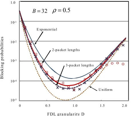
5 . 0

=

ρ against FDL granularity D. The offered load of 5

. 0

=

ρ was selected as a low value, below which the present commercial IP networks are normally operated. The thick solid and dashed lines show the cases for the 2-packet-length and 3-packet-length distributions, and the circles and crosses represent the simulation results for the same respective cases. The thin solid and dashed lines show the results of the fourth order approximations for the exponential and uniform packet-length distributions, respectively.

The lines of the 2-packet-length and 3-packet-length distributions roughly agreed with those of the simulations when D<1.5 , and are situated between those of the exponential and uniform distributions. A realistic packet length distribution would be the shape of the 2-packet-length distribution, overlapping at the low levels with the uniform distribution [19]. Therefore, the blocking probabilities for the realistic distribution are situated between those for the 2-packet-length and the uniform distributions, and are greater than 10-5 for the B=32 and ρ=0.5 case.

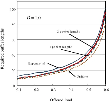
Figure 7 shows the buffer length

B

, at which the blocking probabilities become less than 10-5, against the offered load

ρ

. The FDL granularity

D

was selected to be 1.0 because, in Fig. 4, the blocking probabilities reach the minimum near

0 . 1

=

D . The lines have the same meanings as in Fig. 6. When

B

is small, the permitted offered load values strongly depend on the distributions. When

B

is large, however, the dependency on the distributions decreases. When B=40, permitted offered load values lie in the range greater than 0.5 for the 2-packet-length and uniform distributions. Then, assuming that all-optical packet networks will be operated within the 0.5 offered load, the buffer length

B

is required to be greater than 40.

0 20 40 60 80 100

0.1 0.2 0.3 0.4 0.5 0.6

Offered load

R

eq

u

ir

ed

b

u

ff

e

r

le

n

g

th

s

0 . 1

= D

2 -p a cke t le n gt hs

3-p a cke t len gth s

E xpone n tia l

Un i for m

Fig. 7. Buffer length B, at which blocking probabilities become less than 10-5_{, against offered load ρ. Lines are the same as those in Fig. 6.}

5. Conclusions

This paper established a highly accurate approximation to calculate the blocking probabilities of optical-packet-switch buffers with generally distributed packet lengths. We focused on a simple exponential approximation for tail probabilities of

the steady-state virtual waiting time in the infinite optical buffer. The decay rate of the tail probabilities was asymptotically expanded by a power series of

(

1−ρ′

)

, and approximations up to the fourth order were used for blocking-probability calculations. Calculation values were compared with simulation results.

The main results are as follows.

1)It was clarified that the higher-order terms in the asymptotic expansion reinforced the accuracy of the blocking-probability calculations for all packet-length distributions.

2)By using the fourth order approximation of the decay rate, an accuracy within 10 % was obtained for both the exponential and uniform distribution cases when an offered load is greater than 0.3. For the deterministic distribution case, however, the accuracy was within 60% except for D=0.85~1.25.

3)The approximation was applied to design an optical buffer with realistic IP-network traffic distributions. It was clarified that, assuming that all-optical packet networks will be operated within a 0.5 offered load, the buffer length

B

is required to be greater than 40. The approximations established in this paper can be applied to investigate multiclass optical buffers for priority queueing and to design wavelength-division multiplexing optical packet switches and networks with the maximum throughput.

References

[1] R. S Tucker et al, “Evolution of WDM optical IP networks: A cost and energy perspective,” J. Lightwave Technol., Vol. 27, No. 3, pp. 243-252, 2009.

[2] R. S Tucker, “Scalability and energy consumption of optical and electronic packet switching,” J. Lightwave Technol., Vol. 29, No. 16, pp. 2410-2421, 2011.

[3] F. Callegati, “Optical buffers for variable length packets,” IEEE Commun. Lett., Vol. 4, No. 9, pp. 292-294, 2000.

[4] R. C. Almeida, J. U. Pelegrini, and H. Waldman, “A generic-traffic optical buffer modeling for asynchronous optical switching networks,” IEEE Commun. Lett., Vol. 3, No. 2, pp. 175-177, 2005.

[5] X. Ma, “Modeling and design of WDM optical buffers in asynchronous and variable-length optical packets switches,” Optical Commun., No. 269, pp. 53-63, 2007.

[6] J. Liu, T. T. Lee, X. Jiang, and S. Horiguchi, “Blocking and Delay Analysis of Single Wavelength Optical Buffer with General Packet Size Distribution,” J. Lightwave Technol., Vol. 27, No. 8, pp. 955-966, 2009.

[7] H. E. Kankaya and N. Akar, “Exact analysis of single-wavelength optical buffers with feedback Markov fluid queues,” J. Opt. Commun. Netw., Vol. 1, No. 6, pp. 530-542, 2009.

[9] Y. Murakami, “An approximation for blocking probabilities and delays of optical buffer with general packet-length distributions,” J. Lightwave Technol., Vol. 30, No. 1, pp. 54-66, 2012.

[10] W. Rogiest et al., “Heuristic performance model of optical buffers for variable length packets,” Photon Netw. Commun., Vol. 26, pp. 65-73, 2013.

[11] ITU-T Recommendation Y.1541 (12/2011), Network performance objectives for IP-based services.

[12] L. Kleinrock, “Queueing systems, Vol. 1: Theory”, John Wiley & Sons, New York, 1975.

[13] A. A. Fredricks, “A class of approximations for the waiting time distribution in a GI/G/1 queueing system,” Bell Syst. Tech. J. Vol. 61, pp. 295-325, 1982.

[14] G. L. Choudhury, and W. Whitt, “Heavy-traffic asymptotic expansions for the asymptotic decay rates in the BMAP/G/1 queue,” Stochastic Models, Vol. 10, No. 2, pp. 453-498, 1994.

[15] J. Abate, G. L. Choudhury, and W. Whitt, “Exponential approximations for tail probabilities in queues, I: Waiting Times,” Oper. Res., Vol. 43, No. 3, pp. 885-901, 1995. [16] see 3.6.25 in M. Abramowitz and I. A. Stegun, “Handbook of

Mathematical Functions, 10th printing,” National Bureaus of Standards, U. S. Government Printing Office, Washington, D. C., 1972.

[17] F. Xue et al., “Design and experimental demonstration of a variable-length optical packet routing system with unified contention resolution,” J. Lightwave Technol., vol. 22, no. 11, pp. 2570-2581, 2004.

[18] The cooperative association for the internet data analysis – Packet size distribution comparison between internet links in 1998 and 2008, www.caida.org/research/traffic-analysis/ , 2008.