http://www.sciencepublishinggroup.com/j/ijimse doi: 10.11648/j.ijimse.20170206.11
ISSN: 2575-3150 (Print); ISSN: 2575-3142 (Online)
Development of Methodology for Main Pipelines Linear
Section Stress-Strain State Сhanges Assessment
Liubomyr Zhovtulia, Andriy Oliynyk, Andriy Yavorskyi, Maksym Karpash, Iryna Vashchyshak
Energy Management and Technikal Diagnostic Department, National Technical University of Oil and Gas, Ivano-Frankivsk, UkraineEmail address:
[email protected] (L. Zhovtulia)
To cite this article:
Liubomyr Zhovtulia, Andriy Oliynyk, Andriy Yavorskyi, Maksym Karpash, Iryna Vashchyshak. Development of Methodology for Main Pipelines Linear Section Stress-Strain State Сhanges Assessment. International Journal of Industrial and Manufacturing Systems Engineering. Vol. 2, No. 6, 2017, pp. 66-71. doi: 10.11648/j.ijimse.20170206.11
Received: August 29, 2017; Accepted: September 26, 2017; Published: December 1, 2017
Abstract:
The linear section of main oil and gas pipelines, which are potentially the most dangerous type of pipeline networks, was selected as the object of investigation. A technique for assessing the stress-strain state of the pipeline was developed. Underground pipeline deformation process was mathematically modeled according to the set of points displacement. The process of the underground pipeline points position determination process, estimation of the interpolation accuracy of the underground pipeline spatial position, interpolation step and smoothing parameters determination were described.Keywords:
Pipeline Networks, Stress-Strain State, Methodology, Risk Assessment, Mathematic Model, Axis Coordinates1. Introduction
Pipeline linear part in Ukraine has considerable length and is under constant movement of soil. Statistics of emergencies [1] on pipelines confirm that one of the most dangerous risks of this kind - the risks geodynamic origin, untimely detection of which may result in an emergency.
Movement of the pipe axis causes the change of the stress strain state, critical values of which lead to the destruction of metal.
2. Method
Mathematical modelling of the underground section deformation process
While modelling the process of main pipelines underground sections deformation, based on data of change the spatial configuration of their axis, the approach, suggested for the on-surface pipeline part, is applied. In such a case, using the experimental methods [2, 3, 4], the geometrical configuration of pipeline axis is determined, including the specific accuracy at the control moment of time. It is assumed that the initial position of the pipeline axis is known (for example, according to the design documentation). Thus, for the radius vector of the pipeline
point the following relationship is written.
( , , , ) ( , , , ) ( , , , ) (cos ( , , , ) sin ( , , , ) )
( , , , ) 2
l
l l
l l
r s r t r s r t s r t
s r t b s r t n
D
s r t n
φ φ ρ φ
ω φ ω φ
φ τ
= + ×
× + +
+Ψ −
(1)
where s, ϕ, r - related to the investigated area of underground pipeline, which is simulated as the curved cylindrical body with coordinates respectively:
s - along the pipeline axis; ϕ - by vectorial angle;
l
r - radius vector of the point on the upper generatrix of the pipeline;
D - exernal diameter of the pipeline;
ρ(s, ϕ, r, t); ω(s, ϕ, r, t); Ψ(s, ϕ, r, t) - functions that describe the geometry change of the investigates site, respectively in radial, transverse and longitudinal directions and are either given, or those that are expressed in the process of solving the problem;
l
Τ ; bl; nl - vectors of the tangent binormal and normal to
sin cos
l
x s
r y r
z r φ φ = = = = 1 2 P
R r R D s L
φ ≤ ≤
≤ ≤ ≤ ≤
(2)
where R1; R2 - respectively inner and outer radii of the pipeline;
L - length of the investigated area.
In controlled time moment the dependence (1) is written as:
( ) ( ( ) sin _ ( ) cos ) 2
( ) ( ) ( ( ) sin ( ) cos ) 2
( ) ( ) ( ( ) sin ( ) cos ) 2
n n b
t n n b
n n n
D
x s s s s r
D
r y y s s s s r D
z z s s s s r
α α φ α φ β β φ β φ γ γ φ γ φ = − + = = − + + = − + + (3)
where positions of s, ϕ, r gain the same meaning as in (2), s; ( )
y s ; ( )z s - points position of the upper simulated area, D - pipeline diameter; αn( )s ; βn( )s ; γn( )s - positions of normal vector to the upper generatix; αb( )s ; βb( )s ; γb( )s - position of binormal vector.
When constructing the (3) the following suppositions were used:
Thus, the only output information concerning the geometry change of the underground sections are the coordinates of its’ deformed axle, then in (1) it is assumed that:
}
{
( , , , ) ; ( ); ( )
( , , , ) ( , , , ) ( , , , ) 0
l
r s r t s y s z s s r t r s r t s r t
φ ρ φ ω φ φ ψ φ = = = = (4)
That is due to the fact, that, coordinates of the upper geneatrix are experimentally defined and are set in the form of points position s y si; ( ); ( )i z si , and for origination of ( ; ( ); ( )s y s z s ) interpolation or approximation procedures [6, 7] are used, while there is no information about behavior of
( ; ; ; )s r
ρ φ τ ; ( , , , )ω φ τs r та ψ φ τ( , , , )s r , which makes their record in such a form in which it was written for undeformed areas. If the representation of (3) leads to physically unrealistic results, these functions are simulated by the techniques, listed in [5], where the cross-section configuration change is counted towards the various types of it presentation - ellipticity, pearshape, ellipticity parameter spacing of axle degree of deformability - thus the mentioned methods are justified for surface areas, when the information concerning the crossection damages is available at least visually. In case of underground sections, the representation of (3) is justified with the lack of information concerning the cross-section deformation. This explains the choice of
( , , , )s r 0
ψ φ τ = , as taking into account the underground areas it is also not impossible to perform the visual inspection of the hypothesis justification concerning the flat sections. If the
same methods are used as for the investigation of underground and for surface areas, it is thus at different ways of setting ( ; ; ; )ρ φ τs r ; ( , , , )ω φ τs r ; ( , , , )ψ φ τs r there is one more problem -it is difficult to make the balance equation for underground areas, as it is impossible to take into account in these equations the action of mass forces (weight of the pipe, weight of the product, weight of the soil acting on each section of the pipeline)
Thus, taking into account (2) and (3), the following sequence of calculations is performed:
1. In controlled and initial moment of time the vectors of local basis are defined in each point of simulated area [8]: 0 i k i Э Э t r r ξ ξ ∂ = ∂ ∂ = ∂ (5)
1 s;
ξ = ξ2 =φ;ξ3=r;
1, 2,3
i= ,
where r0 is calculated according to (2), а rt - according to
(3).
Calculating the derivatives are carried out by direct differentiation of (2) and (3) corresponding to the coordinates.
2. Based on (5) the components of metric tensor are defined:
0 0 0 j Э Э
ij i
g = ⋅ , ,j i=1, 2, 3 (6)
k j Э Э
k k
ij i
g = ⋅ , ,i j=1, 2, 3
3. Components q0ij and qkij form matrix, and for the correctness of the calculations the hypothesis should be carried out:
}
{
}
{
0 0 det 0; det 0. ij k k ij G g G g = ≠= ≠ (7)
Performing of (7) based on (6) allow to provide calculations of matrix contravariant components {G0} and
{Gk} as matrix components, inverse to these:
}
{
}
{
1 0 0 0 ; . ij ij ij ij k g g g g − == (8)
0 2
2
2 2
;
( (
)( 2 sin )).
k n n
II b
n
G r
d d
G r g
ds ds
d
R Rr r
ds
β α β
α β
γ
γ φ
=
= − + +
+ − +
(9)
Thus, in case of small strains, the statements of (7) are performed, as in this case:
1
n
d ds
α
<<, d n 1 ds
β
<<, d n 1 ds
γ
<<4. Components of tensor strain are calculated by the [8]:
0 1 1
( ) , 1, 2, 3 2
k ij gij gij i j
ε = − = (10)
5. Based on (5) - (10) the tensor strain components are defined according to Hook’s Law by applying the linear elastic theory device [8]:
( ) 2
ij II gij ij
σ
=λ ε
+µ ε
⋅ (11)The listed calculations can be performed within the model of anisotropic body:
, 1
з
ij ij
k l
Сijkl
σ ε
=
=
∑
⋅ (12)where Cijkl - tensor components of material elastic modulus, although (12) in used only if the pipeline material is substantially anisotropic, and coeficients Cijkl are known. For engineering calculations (11) is typically used, where rl
and xl - material Lame parameters, related to Young's modulus and Poisson coefficient of the material in the following way:
2(1 )
(1 2 )(1 ) E
E µ
σ σ
λ σ σ
=
+
=
− +
(13)
As for pipeline steels, it is generally taken Е=210000 MPa,
σ = 0,3.
In represented (111) function Ι, ( )ε is the first strain invariant and is calculated by the formula:
3 3
0 1 1 , ( ) ij ij
j i
g
ε ε
= =
Ι =
∑∑
(14)where εі is calculated by (10), and gij - according to (8).
Determination of
σ
ij components allows to identify themost dangerous investigating areas, concerning the sector stress state changes, and if at the initial time the pipeline
stress is equal zero, then (11) allows to assess the true strain values. Stress acceptance criterion may be elastic strength value (
σ
пр≈350МПа), or yield strength (σ ≈т 440МПа),in case when the given values are different for various types of piping steels and are determined from the reference literature [9]. It should be mentioned that the described approach to the assessment of the underground stress state is integral, and it does not require the detailed information on loading and stress, the impact of which on the areas is due to displacement measurements. In case, when some tensions (for instance, due to pressure impact, temperature changes, etc.) are acquainted, it is possible to use the superposition principle of elastic theory:
Н B
ij ij ij
σ
=σ
+σ
(15)where
σ
ij - tensions, determined by (11),σ
ijB - acquaintedtensions,
σ
ijН - tensions of unknown nature.3. Position Measurement for
Underground Pipeline Section
Position measurement of pipeline laying, to get its actual position in space and curvature, can be performed by be carried out by non-contact methods by measuring the component of the electromagnetic field created by the alternating current flowing through the pipeline from the low-frequency generator.
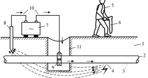
Figure 1. Generalized non-contact determination chart for attitude sensing of underground singular oil and gas pipeline.
1- ground; 2 – oil and gas pipeline; 3 – insulation coating; 4 – damages of insulation coating; 5 – operator; 6 – receiving set of control device; 7 – signal-generator; 8 – ground connection; 9 – collar; 10 - connector; 11 – operational sump
The generalized non-contact determination chart for attitude sensing of underground singular oil and gas pipeline is given in Figure 1.
For control procedure (Figure 1) signal-generator (7) or cathodic protection stations, connecting to the oil and gas pipeline, are used as the current source, and ground connection 8.
finder operation manual. Each determines control point on the pipeline axis is set by the temporary spill or steel pill with given number for further position determination. Location of determined control points shows the pipeline location in sectional view. Pipeline occurrence depth is set in place of pipeline axis determination, usually by pipelines finder, allowing to perform direct occurrence depth measurement. Pipeline occurrence depth hф is set by the formula:
1 2
ф
h =H− ⋅D (16)
where H - distance from the ground surface to the pipeline axis in meters, determined by the pipelines finder. In the absence of pipelines finders, allowing to perform direct pipeline occurrence depth measurement.
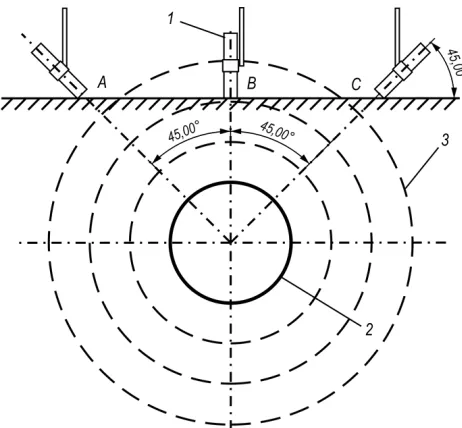
Figure 2. Determination of oil and gas main pipeline occurrence depth.
1 – magnetic antenna of pipelines finder receiving device, 2 – pipeline, 3 – magnetic field lines
The magnetic antenna of the pipeline finder receiver is placed perpendicular to the axis of the pipeline and at the angle of 45° from the vertical axis. By moving the magnetic antenna from the projection of the pipeline axis alternately in different directions, the location of points A and C is determined (Figure 2) by means of minimum volume of the sound signal and/or by the indicator level of pipeline finder receiving device. Distances AB and BC are determined.
Section average АВ and ВС will be equal the distance from the ground surface to the pipeline axis. Oil pipeline occurrence depth hф is determined by the formulae:
1 1
( )
2 2 2
ф
AB BC
h = + − ⋅ = ⋅D AB+BC−D (17)
where D - oil pipeline diameter.
Next step is the determination of space conditions by means of high-precision GPS transmitters. Measurements are performed at fixed checkpoint. The process peculiarity is
summing with the parameter level position of pipeline occurrence depth.
For given investigations the pipelines finder SeekTech SR-60 is used, allowing to determine the location of pipelines axis and occurrence depth with precise accuracy.
The measures data of upper generatix point position and initial pipeline point positions allow to assess the effective stress values.
4. Accuracy Evaluation for Spatial
Attitude Interpolation of
Above-Ground Pipeline Deformed Axle
For realization of the method of stress-strain state assessment, expressed by the dependencies (1)-(13) it is necessary, by means of experimentally measured upper generatix points positions ( sc , ycsi ), ( ))z si to get the
expression for radius vector for every generatix position as
( ; ); ( ))
r= S ycs z s , where y s( ) and z c( ) are continuous functions. For this purpose the widely known interpolation device is used, applying interpolative cubic spline [5, 6] or interpolative cubic spline with test data smoothing. [4]. For interpolative cubic spline the interpolation grid settings are set [10, 11], characterized by the relationships between the minimum and maximum distances between interpolation nodes:
1 2
1 max
3 2 min
max 2
8 3 2
3 3
z h
h f h
ε − ε
= −
′′ (18)
where ε1 - accuracy necessary for interpolating of the
function ( )f x by spline Sf x( ), value of ε sets the accuracy level of function value assignment at interpolation nodes;
2
f′′ - norm of function f′′( )x at given metric space [12]. Dependence (17) can be written in more compact form, taking into account that for main pipelines the radius of axis curvature should meet the hypothesis:
( ) TP
R x ≥ ⋅C D (19)
where DTP- pipeline diameter, C - the constant given by the
value C∈
[
900;1000]
, ( )R x - radius of pipeline curvature, which for engineering calculations can be written in the form:1 ( )
( ) R x
f x =
′′ (20)
3 1 2
1 2 8 z CDTP 3 h
L
ε
−ε
⋅= (21)
2 3 1
1 2 8 z CDTP 3
h
L
ε ε
−
=
(22)
For pipeline section with the length L=100м , pipe diameter DTP =1, 21м with measurement accuracy level 1 sm, step valueh, with which it is necessary to measure the coordinates of the points of the upper generatix, with step
6
h= meters, which is quite acceptable in critical. The interpolation cubic spline peculiarity is the following: at its’ development the accuracy of interpolation setting affects significantly the axis interpolation accuracy. As a rule, the significant deviation from real data yields results that do not correspond to the actual physical picture of the process. The way out is possible by means of implementation of two approaches:
1.Applying the other implementation methods (Lagrange, Chebyshev and Hermite polynomial) or approximation by the LS method, with the resulting curves can differ significantly from real in some cases (insufficient number of interpolation nodes, their inappropriate placement, etc.);
2.Use of approaches, related to embedding the smoothing spline device, allowing to reduce the error of points position measuring by means of some correction coeficients that depend on the accuracy of measuring these points position by testing methods. While embedding the smoothing splice device, the desired smoothing function minimizes on class W22
[ ]
a b;integrated on
[ ]
ab function interval with their square of functional in the form of [6]:10
2 2
0
( ) ( ) ( ( ) )
n
k k k
k a
u U x dx P U x f =
′′
Φ =
∫
+∑
− ɶ (23)Formula (21) requires detailed explanation: fɶk - positions of actually measured points; U x( k) - points positions on the curvature, describing the spline; Pk - weighting coefficients. Minimization problem (21) is solved for different valuesPk. In extreme cases, if Pk → ∞ for any K, then the constructed
spline will not actually be a smoothing, it will pass through all nodes with point positions (xk;fɶk). If Pk →0, then the actually obtained line will be straightforward, since it delivers the extremum of a functional in the form of
2 ( ) ( )
D
a
u U′′ x dx
Φ =
∫
(24)which, obviously, will have a minimum for
( ) 0 ( )
U′′ x = ⇒U x =Ax+B - that is, U x( ) - straightforward
line. With the knowing of performed measurements accuracy
k
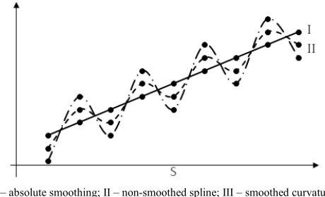
f , it is possible to get the values Pk, where in the function configuration U x( ) will, from the one hand, smooth the effect of measurements error, and from the other hand, will not allow to lose the features of the real section configuration. This can be depicted as simulation in the following way (Figure 3)
I – absolute smoothing; II – non-smoothed spline; III – smoothed curvature
Figure 3. Test data smoothing.
Optimizing methods (24) with parameters Pk , which characterize the level of data smoothing depending on the measurement accuracy, are well-known, and they are used for above-ground sections [5], for this reason their application for underground sections is well-reasoned. In particular, the procedure of functional minimizing (23) is used, by implementation of iteration procedure, at each step of which the coefficients are based on the formula:
( ) ) ( )
( 1) (
j
k k
j j
k k
U x y
P P
ε
+ = ⋅ −ɶ (25)
which is realized until the fulfillment of the condition is achieved
( )( )
1
j
k k
U x y
ε
−ɶ →
(26)
In formulae (25), (26) j - iteration process step number;
ε - accuracy of node points position measurement, Pk( )j - smoothing coefficient value at iteration process step j ,
( )
j k
U x - smoothed positions of node point Xk after
minimizing procedure (23) at iteration process step under number j; yk - initial non-smoothed positions of this node point. Test calculations within implementation of these method show, that by the embedding this smoothing iteration procedure, the error of stress evaluation is 5± MPa for the operating pipeline section, displacement measurement of which is carried out with the accuracy of 1 mm for the pipeline section with the L=100м.
5. Conclusion
the process of pipeline deformation for the assessment, namely assessment of the existing values and prediction of stresses. The method of evaluation of the pipeline stress-strain state is developed. The process of the underground section of the pipeline deformation is mathematically developed according to the data of the displacement of a certain set of points. The determination process of underground pipeline underground pipeline points position, interpolation accuracy evaluation of the of the above-ground pipeline deformed axis spatial and determination process of interpolation step and smoothing parameters were described.
The conducted investigations allow to estimate the underground section of main pipeline stress-strain state by the non-contact method. The authors plan to continue the study the pipelines’ stresses assessment, subject to soil landslide
References
[1] Gas pipeline incidents. 8-th Report of the European Gas Pipeline Incident Data Group (1970-2010). Access mode: (http://www.egig.nl/downloads/8th_report_EGIG.pdf). [2] V. Y. Bash. Stress and deformation analysis by thermoelectric
technique / V. Y. Bash. - Kyiv: Naukova dumka, 1984. - 100 p. [3] V. A. Zolochevsky. Experiments in development mechanic / V.
A. Zolochevsky. - Moscov: Stryizdat, 1983. - 192 p.
[4] V. V. Kluev. Non-destructive testing and diagnostics / V. V. Kluev. - Moscov: Mashynostroenie, 2003. - 656 p. - (3). [5] A. P. Oliynyk Mathematical models for process of
quasy-stationary deformation of pipline and industrial systems under their spatial configuration change [Text] / A. P. Oliynyk // Scientific publication. - Ivano-Frankivsk: IFNTUOG, 2010. - 320 p.
[6] A. A. Samarsky. Numerical procedures: College-level study guide / A. A. Samarsky, A. V. Gulin. - Moscov: Nauka. MEO of physical and mathematical literature, 1989. - 432 p. [7] G. I. Marchuk. NUMERICAL METHEMATICS
PROCEDURES / G. I. Marchuk. - Moscov: Nauka, 1984. - 608 p.
[8] L. I. Sedov. Continuum mechanics / L. I. Sedov. - Moscov: Nauka, 1984. - 572 p.
[9] SNiP 2.05.06-85. Main pipelines / Gosstriy SSSR. - М.: CPTE Gosstroy SSSR, 1999. - 125 p.
[10] N. P. Korneychuk. Extremal problems in approximation theory / N. P. Korneychuk. - Moscov: Nauka, 1976. - 320 p. [11] N. P. Korneychuk. Splines in approximation theory / N. P.
Korneychuk. - Moscov: Nauka, 1984. - 422 p.