Open Access
Methodology
Enhancing the comparability of costing methods: cross-country
variability in the prices of non-traded inputs to health programmes
Benjamin Johns*
1, Taghreed Adam
2and David B Evans
2Address: 1Health System Financing (EIP/HSF), World Health Organization, 9th Floor Bina Mulia – I Building, Jl Rasuna Said Kav. 10, Kuningan
Jakarta 12950, Indonesia and 2Health Systems Financing (EIP/HSF), World Health Organization, Geneva, Switzerland
Email: Benjamin Johns* - [email protected]; Taghreed Adam - [email protected]; David B Evans - [email protected] * Corresponding author
Abstract
Background: National and international policy makers have been increasing their focus on developing strategies to enable poor countries achieve the millennium development goals. This requires information on the costs of different types of health interventions and the resources needed to scale them up, either singly or in combinations. Cost data also guides decisions about the most appropriate mix of interventions in different settings, in view of the increasing, but still limited, resources available to improve health.
Many cost and cost-effectiveness studies include only the costs incurred at the point of delivery to beneficiaries, omitting those incurred at other levels of the system such as administration, media, training and overall management. The few studies that have measured them directly suggest that they can sometimes account for a substantial proportion of total costs, so that their omission can result in biased estimates of the resources needed to run a programme or the relative cost-effectiveness of different choices. However, prices of different inputs used in the production of health interventions can vary substantially within a country. Basing cost estimates on a single price observation runs the risk that the results are based on an outlier observation rather than the typical costs of the input.
Methods: We first explore the determinants of the observed variation in the prices of selected "non-traded" intermediate inputs to health programmes – printed matter and media advertising, and water and electricity – accounting for variation within and across countries. We then use the estimated relationship to impute average prices for countries where limited data are available with uncertainty intervals.
Results: Prices vary across countries with GDP per capita and a number of determinants of supply and demand. Media and printing were inelastic with respect to GDP per capita, with a positive correlation, while the utilities had a surprisingly negative relationship. All equations had relatively good fits with the data.
Conclusion: While the preferred option is to derive costs from a random sample of prices in each setting, this option is often not available to analysts. In this case, we suggest that the approach described in this paper could represent a better option than basing policy recommendations on results that are built on the basis of a single, or a few, price observations.
Published: 24 April 2006
Cost Effectiveness and Resource Allocation 2006, 4:8 doi:10.1186/1478-7547-4-8
Received: 22 July 2005 Accepted: 24 April 2006
This article is available from: http://www.resource-allocation.com/content/4/1/8
© 2006 Johns et al; licensee BioMed Central Ltd.
Introduction
Cost and cost-effectiveness studies are increasingly being used to guide practical policy decisions in many parts of the world. This tendency has received additional impetus in low income countries with international attention focused on how best to achieve the health-related millen-nium development goals (MDGs). The numerous result-ing studies explore the impact of different mixes of interventions on health as well as the resource require-ments to scale them up to the extent necessary to achieve the goals [1-4].
Costing and cost-effectiveness studies have, however, fre-quently included only the costs incurred at the point of delivery to beneficiaries, omitting those incurred at other levels of the system. These additional costs have been defined elsewhere as programme costs and we use that ter-minology in this paper [5]. They include the costs of establishing and running a programme at national, pro-vincial or district administrative levels, for activities such as planning and supervision, advertising and media, and training.
In some published studies it is not clear whether pro-gramme costs have been included. Where they are included it has been common to assume that they are an arbitrary proportion of total costs – commonly 10% – although at other times programme costs estimated from other countries have been converted to the local setting at official or purchasing power parity (PPP) exchange rates [6]. The few studies that have attempted to estimate pro-gramme costs directly have shown that they vary by inter-vention and can range from a relatively low to a substantial proportion of total costs [7,6]. The total exclu-sion of programme costs, or inaccurate estimation meth-ods, can misrepresents the resources required to implement or maintain health interventions and biases comparative assessment of their cost-effectiveness. In its CHOICE project [9], WHO seeks to assist countries to set priorities by making publicly available region- and country-specific estimates of the costs, effectiveness, and cost-effectiveness of a large set of interventions, analysed in a standardized and comparable way [10]. The project was developed in response to the recognition by countries that it is not feasible for each of them, particularly those with limited capacity, to perform full analyses of the cost-effectiveness of all possible ways of spending scarce health resources in their settings. Subsequently, WHO-CHOICE has also provided assistance to global and country efforts to estimate the resources required to scale up health inter-ventions, including those aimed at achieving the millen-nium development goals [11]. In this work, WHO has sought to include programme costs as accurately as possi-ble and in a standardized way, in addition to the costs
incurred in providing services directly to patients – e.g. for pharmaceuticals, investigatory tests, outpatient visits and hospital stays.
An ingredients approach to costing has been used where the physical quantities of the necessary inputs are multi-plied by their unit prices to obtain total costs. To facilitate this work, data have been collected on the unit costs or prices of the different types of inputs and activities used in key interventions for as many countries as possible. This has revealed that unit costs vary considerably both within and across countries. For this reason, the common prac-tice in cost-effectiveness studies of basing cost estimates on a single observation of the cost of an input – for exam-ple, the price of labour, transportation or renting an office – can lead to misleading results [6]. This has already been illustrated by Adam et al. [10] for hospitals where the cost per inpatient day was shown to vary by an order of mag-nitude across hospitals within the same country. If an ana-lyst were to use the unit cost estimated for a hospital that happens to be an outlier, high or low, the results would be biased either against or towards hospital-based interven-tions. Moreover, it would not be possible to know the direction or extent of any possible bias.
For this reason, we have tried to explore alternative ways of obtaining average unit costs for cost-effectiveness anal-ysis aimed particularly at countries where there are limited data points available from accurate costing studies. Clearly the first and best solution would be to base costs on a representative sample of observations for all possible inputs and activities, but rarely do analysts have access to these data or the funds to generate them, even in the rich-est countries.
Results for inpatient days and outpatient visits to hospi-tals have already been published [10] and those for department-specific hospital stays and labour costs are under review [10,12-14]. This paper describes models focusing on two "non-traded" inputs to programme costs – media and advertising for health promotion, and utili-ties such as water and electricity that are essential ingredi-ents of most health programmes. Media can be a very small or a very large component of costs, at the limit approaching 100% of costs for mass media campaigns for health promotion, for example. Utilities, on the other hand, are almost always present but rarely constitute a large part of costs.
they are the most important non-traded inputs for all interventions.
The remaining two objectives are specific to these two inputs. The second objective is to understand the determi-nants of variations in the unit costs of these inputs across and within countries. The third is to use the estimated relationships to impute an average cost for each country, taking into account the observed variation, uncertainty, and the levels of the other determinants. It is postulated that this average cost is likely to be a more appropriate unit price to use in an economic analysis than a single observation that might well be an outlier.
The paper has, therefore, two audiences. The first consists of analysts who conduct or interpret costing and cost-effectiveness studies. The second comprises researchers and policy makers seeking to understand the methods that have been used in the WHO-CHOICE project. The paper is organized as follows. For each of the two inputs (media and utilities) the methods and results are presented in turn, including the imputed prices using the best-fit model for a selected number of countries. We con-clude with an overall discussion of the potential uses of these results for policy.
Methods and results
Theoretical considerationsWhere a good is traded internationally and no producer or consumer is sufficiently large to influence price, the pur-chase price (free on board or fob) available to all import-ing countries should be the same [15]. Differences in unit costs observed across countries would, under these cir-cumstances, be attributable to differences in transport, insurance and internal distribution costs. Many inputs to health are traded internationally and the markets are approximately competitive – examples are generic phar-maceuticals and items of medical equipment where there are many alternative suppliers. In this case there would be a single internationally competitive price which would reflect the marginal cost of production and the marginal value to the international consumer of the last unit pur-chased.
On the other hand, the market for brand name pharma-ceuticals is not competitive with different purchasers being able to negotiate different prices with the monopoly producers [15]. There could be numerous international prices for inputs such as these, determined partly by a country's capacity to pay and its bargaining power. Price will certainly be above the marginal costs of production [16] and variations in prices across countries would be expected to be positively correlated with GDP per capita or some other measure of ability to pay.
Where goods are not traded internationally, the interac-tion of domestic supply and demand influences price. Assuming that no producer or consumer is sufficiently large to influence price and that the government does not intervene, price would be the point where the domestic supply and demand curves intersect, or where the ginal valuation of benefit by consumers equals the mar-ginal cost of production. When the good is an input to production, such as cement for building, or paper for printing, competitive markets would imply that price is equal to the marginal cost of production (which deter-mines the supply curve) as well as the value of the mar-ginal product produced (which determines the demand curve).
The demand curve would shift outwards with increases in GDP per capita because of the income effect. Given that wages for most types of labour are positively correlated with GDP per capita, [17] the supply curve would shift upwards as GDP per capita increases – e.g. each unit of output would cost more in richer countries. Taken together, and assuming away, for the moment, other influences on prices such as differences in production technologies, the price of pure non-traded goods would be positively correlated with GDP per capita.
The interaction of supply and demand described above assumes that production technology does not change across countries with increases in GDP per capita. If, for example, there are economies of scale and the long run average cost curve continues to fall with increases in out-put, countries with larger markets could be operating on different short run average and marginal cost curves asso-ciated with different scales of production [18]. Countries with smaller markets would be seen to have supply curves that are above those of countries with larger markets, and thus have higher prices than larger markets. Accordingly, although a positive relationship would still be expected between the price of pure non-traded goods and GDP per capita on average, the relationship might not be found if significant economies of scale in production existed – something that is possible with utilities in particular.
coun-tries would be more strongly or weakly correlated with variations in GDP per capita.
The two "non-traded" inputs under discussion here are really intermediate factors of production. They are inputs to the production of health, but in turn require physical inputs such as labour, equipment, and raw materials. Some of these are traded internationally, while others are not (and thus, the goods under discussion are not 'pure' non-traded goods). Market structures differ as well. Media outlets and utilities are sometimes owned by government, with little or no competition. In other cases the producing companies are privately owned and operated, usually with some market power to affect prices. Their ability to do so depends on the extent and nature of government regulation and control.
While we would still expect that prices will vary across countries with national ability to pay and variation in the costs of production, both positively correlated with national income or GDP per capita where markets are approximately competitive, the strength of the relation-ship would still be moderated by differences in domestic market conditions across countries and the extent to which the two non-traded intermediate inputs themselves use traded factors of production. At the extreme, however, if governments effectively set prices for utilities or for media outlets, it is not clear what type of relationship would be observed.
Accordingly, we hypothesize here that a positive relation-ship would be expected between GDP per capita and unit price except in the case of pure traded goods where prices should not differ very much across settings. However, we recognize that the strength of this relationship would depend on a number of factors influencing supply and demand including the extent to which our intermediate inputs use traded primary factors of production and the extent of market regulation or control by government. At the extreme, if governments control prices directly, it is possible that a negative relationship, or no relationship, would be observed depending on the principles driving their pricing policies.
Data collection
In the course of 2000–2001, the WHO-CHOICE project hired 19 consultants from different countries chosen to span different epidemiological and income regions of the world. A workshop demonstrated a standardized cost data collection tool (CostIt) and a detailed list of ingredients or inputs to the various activities required to develop or maintain a programme or intervention. This was designed to increase the comparability of data-collection methods across interventions and countries, and to reduce meas-urement error (for more information see [7]).
In addition to the data collected by the consultants, data from a variety of additional sources were identified and added to the data set. These are described separately for the two categories of non-traded inputs subsequently. All of the data were examined for outliers. When outliers were detected, the observation was checked to ensure that it had been entered accurately. In a few cases, outliers lack-ing a plausible explanation were eliminated. The data were entered into STATA software, which was also used for the analysis [23].
The following sections describe the data, model specifica-tion and results for the two programme cost inputs in turn. Tests for goodness of fit, retransformation methods, estimation of predicted values and uncertainty intervals are only presented after the first model as they are the same for all models.
1. Flyers, posters, and advertising Data
Various forms of information dissemination are critical to health promotion but are also used to provide informa-tion to populainforma-tions about the availability of curative or preventive activities such as immunization days. It can be divided into two broad categories: printed materials for distribution, and the use of advertising time or space in media outlets such as radio, television and newspapers. For the former, informational flyers and posters were taken as representative of the broader category. To main-tain cross-country comparability of prices, flyers were defined as one A4 or comparable sheet of paper printed on both sides, and posters were defined as one square metre. The costs of media advertising were based on one minute of television, one minute of radio (both during daytime but not prime time), and a quarter page adver-tisement in the body (i.e. not the front or last page) of a newspaper.
analysis, by applying consumer price indices (CPI) from central-bank or similar government agency web-sites, or CPIs from international organizations when the central bank did not report them.
Model specification
Separate regressions were run for printed material and advertising in the mass media. The dependent variable in both is unit cost as a percentage of GDP per capita. Using a percentage allows costs to be analysed in a metric easily converted into all currency units. The first explanatory var-iable is GDP per capita as described above, which was tested in terms of both international dollars (denoted by the symbol I$ – converted from domestic currency to I$ using purchasing power parities) and US dollars (US$ – converted at official exchange rates). (For prediction pur-poses, it makes no difference whether the dependent var-iable is the ratio of price to GDP or simply the price itself – mathematically, the elasticity of price to GDP per capita is simply our beta coefficient plus unity e.g. 1+β. This is discussed further in the results section.)
A variety of regional dummies were tested to see if there were region-specific characteristics that might influence prices. We hypothesized that countries that were geo-graphically contiguous were more likely to have interre-lated markets and similar price structures, so tested the following regional dummies: sub-Saharan Africa, Latin America, Europe, Eastern Mediterranean/Middle-east, Asia, Oceania and North America. At different times the dummies for Asia were further subdivided into "South Asia" and "Eastern Asia" and Europe was divided into Eastern and Western Europe. As an alternative, we also tested grouping countries into those that were developed and less developed, and explored other income classifica-tory systems such as that utilized by the World Bank. For media advertising, we had more than one data point from a number of countries. To correct for the possible interdependence of the error terms because of this cluster-ing, the regressions were re-run using the robust (cluster) option in STATA, based on the Huber-White method of robust variance estimation [23]. In this case, the coeffi-cients are identical to those in OLS regressions, but the variance, and therefore the significance, of the coefficients can differ.
Third, a number of factors reflecting the domestic supply and demand for advertising time and space were consid-ered. These included the size of the population in the serv-ice area which is likely to make advertising more attractive and raise demand, and therefore prices [24]. A variant of this, the predicted market size (MS), which takes into account the number of people with access to the particular form of media, was also tested [25,26]. It is calculated as:
MSi = PSi * PAi, (Equation 1)
where PSi is the population of the area served by the media outlet in the area where the ith observation is found, and PAi is the percentage of the population with access to the media outlet. For television and radio, we used the proportion of people with television or radio[27] as a proxy for access, and the adult literacy rate was used for newspapers [28].
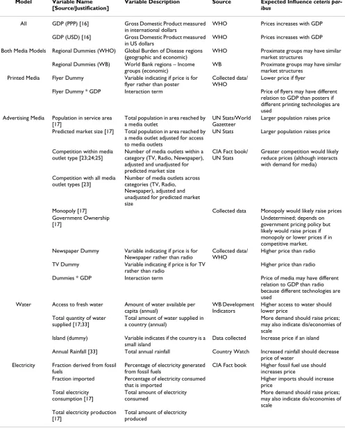
On the other hand, the extent of competition between media outlets would likely reduce prices, so the extent of competition in the market was also tested as an explana-tory variable. Competition was tried first as the number of outlets per potential market audience. This assumes that newspapers, televisions, and radio outlets do not compete with one another. Because there is some evidence that print, radio, and television advertising is substitutable, the extent of competition between all forms of media was also tested [28]. Dummy variables indicating monopoly of the market and whether the government owned or operated the media outlet (where unit costs could be higher or lower than private sector outlets) were also tested as fac-tors influencing the nature of the interaction between sup-ply and demand. Table 1 summarizes the explanatory variables used at various times in each of the models.
Ordinary least squares (OLS) regression was used in the analysis. After exploring the model variables for non-line-arity and experimenting with possible transformations, the natural log transformation was used for both the dependent and the explanatory variables that showed evi-dence of non-linearity, since this form best approximated a normal distribution of the variables. It is shown in Equa-tion 2:
where ln denotes natural logarithms, UCi is the unit cost (poster, flyer, or advertisement) in the ith country in year 2000 and GDPi is the GDP per capita of the ith country in 2000. In all equations, X1 is the natural log of GDP per capita in 2000 of the country where the ith observations is located and e denotes the error term. Regional dummies were included as explanatory (X) variables in all equa-tions as were possible interacequa-tions between these dum-mies and GDP per capita.
For posters and flyers, the only additional explanatory var-iable included in the equation was a dummy varvar-iable indicating that the observation was for a flyer rather than a poster. The effect of interacting this variable with GDP per capita was also explored.
ln UC GDPi/ i iXi ei, i
n
(
)
= + +(
)
=
∑
α0 α1
Table 1: Independent variables explored for each model
Model Variable Name [Source/Justification]
Variable Description Source Expected Influence ceteris par-ibus
All GDP (PPP) [16] Gross Domestic Product measured in international dollars
WHO Prices increases with GDP
GDP (USD) [16] Gross Domestic Product measured in US dollars
WHO Prices increases with GDP
Both Media Models Regional Dummies (WHO) Global Burden of Disease regions (geographic and economic)
WHO Proximate groups may have similar market structures
Regional Dummies (WB) World Bank regions – Income groups (economic)
WB Proximate groups may have similar market structures
Printed Media Flyer Dummy Variable indicating if price is for flyer rather than poster
Collected data/ WHO
Lower price if flyer
Flyer Dummy * GDP Interaction term Price of flyers may have different
relation to GDP than posters if different printing technologies are used
Advertising Media Population in service area [17]
Total population in area reached by a media outlet
UN Stats/World Gazetteer
Larger population raises price
Predicted market size [17] Total population in area reached by a media outlet adjusted for access to media outlets
UN Stats Larger population raises price
Competition within media outlet type [23;24;25]
Number of media outlets within a category (TV, Radio, Newspaper), adjusted and unadjusted for predicted market size
CIA Fact book/ UN Stats
Greater competition would likely reduce prices (although interacts with demand for media)
Competition with all media outlet types [23]
Number of media outlets across categories (TV, Radio,
Newspaper), adjusted and unadjusted for predicted market size
Monopoly [17] Collected data Monopoly would likely raise prices
Government Ownership [17]
Undetermined; depends on government pricing policy but likely would raise prices if monopoly or lower prices if in competitive market.
Newspaper Dummy Variable indicating if price is for Newspaper rather than radio
Collected data/ WHO
Higher price than radio
TV Dummy Variable indicating if price is for TV rather than radio
Higher price than radio
Dummies * GDP Interaction term Price of media may have different
relation to GDP than radio because different technologies are used
Water Access to fresh water Amount of water available per capita (annual)
WB Development Indicators
Higher access to water should lower price
Total quantity of water supplied [17;33]
Total amount of water supplied in a country (annual)
More demand should raise prices; may also indicate dis/economies of scale
Island (dummy) Variable indicates if the country is a small island
Data collected Increase price if an island
Annual Rainfall [33] Total annual rainfall Country Watch Increased rainfall should decrease price of water
Electricity Fraction derived from fossil fuels
Percentage of electricity generated from fossil fuels
CIA Fact book Higher fossil fuel use should increases price
Fraction imported Percentage of electricity consumed that is imported
Higher imports should increase price
Total electricity consumption [17]
Total amount of electricity consumed
More demand should raise prices; may also indicate dis/economies of scale
Total electricity production [17]
For advertising time and space, in addition to the varia-bles described above, a dummy variable was included for observations relating to newspapers, and another for those relating to television advertising. In interpreting the coefficients, the base case was, therefore, radio advertis-ing.
Goodness of fit
Standard regression diagnostic procedures were used to check all models, including those in subsequent sections, for misspecification and goodness of fit. These procedures included exploration of the correlation between inde-pendent variables; estimation of the tolerance test and its reciprocal variance inflation factors (VIF) for multicolline-arity; visual inspection of residual plots and statistical assessment for non-linearity and heteroskedasticity; and the Breusch-Pagan test for heteroskedasticity [23].
Imputing average prices and uncertainty analysis
Once the equations explaining variation in unit costs had been estimated, two types of uncertainty need to be con-sidered when they are to be used to predict prices for the different settings. Uncertainty in the α and β coefficients of equation 2 derives from having the fact that the equa-tion is estimated from a sample of observaequa-tions from the entire possible data set; fundamental uncertainty occurs because the independent variables do not explain all of the variation in the dependent variable [29]. To account for these types of uncertainty, statistical simulation fol-lowing the logic of survey sampling is used to impute average unit costs, standard deviations, and confidence intervals. The methods used to determine predicted values
and uncertainty ranges have been described in detail else-where [10] and are summarized briefly here.
Two steps are involved. First, simulated parameter values are obtained by drawing random values from the normal distribution of the estimated parameters using their vari-ance co-varivari-ance matrix to obtain a new value of the parameter estimate. This is repeated 1000 times. Second, simulated predicted values of ŷ (the quantity of interest) are calculated, as follows: (1) one value is set for each explanatory variable; (2) taking the simulated coefficients from the previous step, the systematic component (g) of the statistical model is estimated, where g = f (X, B), this results in 1000 values of g; (3) the predicted value "ŷ" is simulated by taking a random draw from the systematic component of the statistical model, this is repeated 1000 times to produce 1000 predicted values, thus approximat-ing the entire probability distribution of ŷ. From these simulations, the mean predicted value, standard devia-tion, and 95% confidence interval around the predicted values are computed. In this way, this analysis accounts for both fundamental and parameter uncertainty. Since the predicted values are estimated in natural loga-rithms, simply taking the anti-log of these values to retransform them to natural units results in a biased esti-mate because it provides the median, not the mean, val-ues. This bias is due to the model variables having a normal distribution in log scale, which is not the case in natural units. Duan 1983 presented a solution to this bias, called the smearing factor, and is applied here [30]. This is done by multiplying the antilog of the estimated values by the smearing factor, which is the mean of the antilog of the model residuals. Separate smearing factors were calcu-lated for each regression equation, as reported in Table.
Results
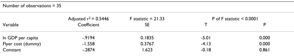
Table 3 shows the result of the best fit model for posters and flyers. The only statistically significant variables are GDP per capita and the dummy for flyers (versus posters). The fit of the model was better using GDP per capita in
Table 3: Results of regression for printed materials
Number of observations = 35
Adjusted r2 = 0.5446 F statistic = 21.33 P of F statistic < 0.0001
Variable Coefficient SE T P
ln GDP per capita -.9194 0.1835 -5.01 0.000
Flyer cost (dummy) -1.558 0.3767 -4.13 0.000
Constant -.2874 1.623 -0.18 0.861
Dependent variable: log ratio of price of printed materials to GDP per capita Breusch-Pagan test of heteroskedasticity: 1.02 (p = 0.31 (Chi2)).
VIF test for multicolinearity:1.02 (less than 2 indicates no multicollinearity)
Table 2: Smearing factor for each regression model
Model number Input explored Smearing factor
1a Printed media 1.693
1b Advertising media 2.334
2a Water 1.249
international dollars rather than in US dollars using offi-cial exchange rates. This was true for all subsequent mod-els. The adjusted R squared is 0.54, with an F statistic of 21.33 (p < 0.0001), indicating that the model explains more than half of the variation of the cost of printed media across countries.
The coefficient for GDP per capita is negative and its abso-lute value is just less than one (-0.92, p < 0.0001). This is the elasticity of the dependent variable with respect to a change in GDP per capita, suggesting that a 1% increase in GDP per capita results in a fall in the ratio of the unit cost of posters and flyers to GDP per capita of 0.92%. The elas-ticity of unit price (as opposed to the ratio) with respect to GDP per capita is 1+β, as shown earlier, or 0.09 in this case. Unit costs of printed material are, therefore, inelastic with respect to GDP per capita – they rise as GDP per cap-ita rises, but at a much lower rate than GDP per capcap-ita. The dummy variable indicating whether the price is for a poster or flyer (flyer = 1) has a negative coefficient and indicates that the price of a flyer is approximately 21% of the price of a poster (p < 0.0001). None of the interactions proved to be significant.
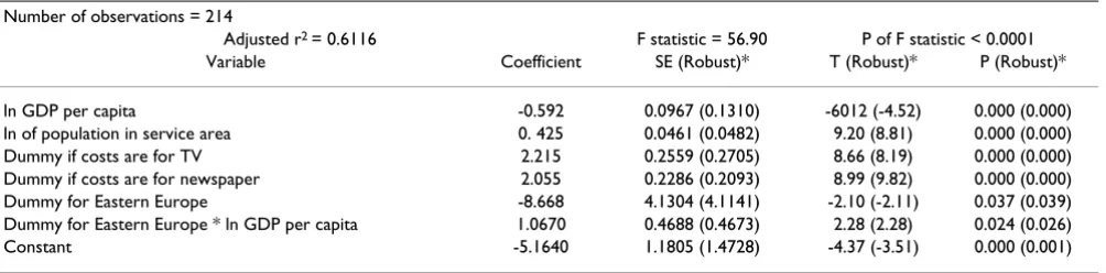
Table 4 presents the best fit results for media advertising using the robust cluster option. The independent variables explain a greater share of the variation in the price ratio than they do for posters and flyers (R squared = 0.61) and the F statistic is high and significant (F = 56.9; p < 0.0001). There are no problems with multicollinearity or heter-oskedasticity, and all variables remain significant after controlling for clustering.
The relationship of unit cost to GDP per capita is more complex than for the printed materials because of the interaction variables, and the elasticises (of price, not the ratio) derived from the equation are summarized in Table 5.
All prices increase with GDP per capita. Unit prices are lower than would be expected for the level of national income in Eastern Europe (the coefficient for the regional dummy is negative and significant), but prices rise with GDP/capita more rapidly than in the rest of the world. In fact, price is elastic in Eastern Europe and inelastic in the rest of the world.
Prices are also positively correlated with the size of the population in the service area, in this case probably reflecting the fact that advertisers are willing to pay more if they reach more people rather than indicating disecon-omies of scale in covering a wider population. The varia-bles for media outlets per potential audience were significant only when size of the population served is not included in the equation; the two variables also showed relatively high correlation (0.63). Since the size of the population served was found to be more significant, only this variable was retained in the equation. None of the other supply or demand variables proved to be significant in the best equation.
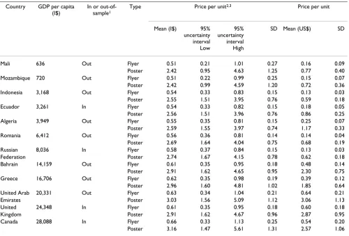
Imputing average prices per country
Table 6 and Table 7 report the imputed average prices for each country based on the reported equations and the methods described earlier, in year 2000 International (I$) and US dollars (US$). Standard deviations and 95% con-fidence intervals for each estimate are also provided. Full details for all countries and regions are available at [9].
Table 5: Elasticises of the unit price of advertisements with respect to GDP per capita
Eastern Europe Rest of the World
Media 1.475 0.408
Table 4: Results of regression for advertising time or space
Number of observations = 214
Adjusted r2 = 0.6116 F statistic = 56.90 P of F statistic < 0.0001
Variable Coefficient SE (Robust)* T (Robust)* P (Robust)*
ln GDP per capita -0.592 0.0967 (0.1310) -6012 (-4.52) 0.000 (0.000)
ln of population in service area 0. 425 0.0461 (0.0482) 9.20 (8.81) 0.000 (0.000)
Dummy if costs are for TV 2.215 0.2559 (0.2705) 8.66 (8.19) 0.000 (0.000)
Dummy if costs are for newspaper 2.055 0.2286 (0.2093) 8.99 (9.82) 0.000 (0.000)
Dummy for Eastern Europe -8.668 4.1304 (4.1141) -2.10 (-2.11) 0.037 (0.039)
Dummy for Eastern Europe * ln GDP per capita 1.0670 0.4688 (0.4673) 2.28 (2.28) 0.024 (0.026)
Constant -5.1640 1.1805 (1.4728) -4.37 (-3.51) 0.000 (0.001)
*The results as reported after a robust and country clustering are reported in the parenthesis. Dependent variable: log ratio of price of media and advertising to GDP per capita
Breusch-Pagan test of heteroskedasticity: 1.91 (p = 0.1667 (Chi2)).
2. Utilities Data
The three main categories of utilities used in the produc-tion of health services across countries are electricity, water, and telephone-based communications. The price of electricity was standardised at the cost of one kilowatt-hour (KWh) and for water, at one cubic metre. The sources of data for electricity included, in addition to the 19 con-sultants, the United States Department of Energy, the World Energy Organization and the Governments of South Africa, Namibia, and Botswana for their respective countries [31,32]. This resulted in a data set on prices from 60 countries. The WHO and UNICEF Joint Monitor-ing Programme for Water Supply and Sanitation under-took an extensive survey of the cost of water for a large number of countries, resulting, together with the consult-ant data, in a data set from 86 countries for water. The International Telecommunications Union publishes the costs of local telephone calls for all but a handful of
countries [33]. The published rates are often standardised at the national level, so we simply took these data for WHO-CHOICE rather than attempting to develop our own models. Telecommunication costs are not, therefore, discussed further in this paper.
Model specification Water
The OLS regression specification is the same as Equation 2 above, where the dependent variable is the ratio the unit cost of a cubic metre of water in the country covered by the ith observation, in year 2000 prices, divided by GDP per capita in that year. X1 is again GDP/capita, as in all the models. To reflect demand [34], access to fresh water and the total quantity supplied were tested as explanatory var-iables, although the latter might also indicate the exist-ence of economies or diseconomies of scale on the supply side [35]. Two purely supply side variables were explored [34] – a dummy variable indicating if the country is a small island, and annual rainfall [36]. Small islands have
Table 6: Estimated price for print media for selected countries in 2000 I$ and US$
Country GDP per capita (I$)
In or out-of-sample1
Type Price per unit2,3 Price per unit
Mean (I$) 95%
uncertainty interval Low
95% uncertainty interval High
SD Mean (US$) SD
Mali 636 Out Flyer 0.51 0.21 1.01 0.27 0.16 0.09
Poster 2.42 0.95 4.63 1.25 0.77 0.40
Mozambique 720 Out Flyer 0.51 0.22 0.99 0.25 0.15 0.07
Poster 2.42 0.99 4.59 1.20 0.72 0.36
Indonesia 3,168 Out Flyer 0.54 0.33 0.83 0.15 0.13 0.03
Poster 2.55 1.51 3.95 0.76 0.59 0.18
Ecuador 3,261 In Flyer 0.54 0.33 0.82 0.15 0.18 0.05
Poster 2.56 1.51 3.96 0.76 0.86 0.25
Algeria 3,949 Out Flyer 0.55 0.35 0.81 0.15 0.25 0.07
Poster 2.59 1.55 3.97 0.74 1.17 0.33
Romania 6,412 Out Flyer 0.56 0.36 0.81 0.14 0.14 0.04
Poster 2.69 1.64 4.04 0.75 0.68 0.19
Russian 8,036 In Flyer 0.58 0.37 0.84 0.15 0.13 0.03
Federation Poster 2.74 1.67 4.15 0.78 0.62 0.18
Bahrain 14,159 Out Flyer 0.61 0.35 0.95 0.18 0.48 0.14
Poster 2.91 1.62 4.65 0.95 2.30 0.75
Greece 16,706 Out Flyer 0.62 0.35 0.98 0.19 0.39 0.12
Poster 2.96 1.60 4.81 1.02 1.85 0.64
United Arab 20,331 Out Flyer 0.63 0.34 1.04 0.21 0.64 0.21
Emirates Poster 3.03 1.56 5.09 1.12 3.06 1.13
United 24,348 In Flyer 0.61 0.35 0.95 0.18 0.60 0.18
Kingdom Poster 2.91 1.62 4.67 0.96 2.87 0.95
Canada 28,088 In Flyer 0.66 0.33 1.13 0.25 0.54 0.20
Poster 3.16 1.47 5.61 1.31 2.57 1.06
1In and out of sample indicate whether or not the country was included in the data set used to estimate the model. 2Regional estimates are available at http://www.who.int/choice.
more rapid run-off rainfall and less capacity to store water than other settings. All continuous variables were incor-porated in natural logarithms as described earlier.
Electricity
A body of literature exists explaining variation in the price of electricity on daily or spot markets, where markets have been deregulated [37-41]. However, short term fluctua-tions are more volatile than longer run changes, although
this literature helps identify possible explanatory varia-bles [42-44]. Following equation 2, X1 is again GDP/cap-ita. The percentage of electricity generated from fossil fuels in the country [45] and the fraction of total consumption derived from imported electricity were used to reflect sup-ply conditions. In the absence of economics or disecono-mies of scale, the ratio of price to GDP is expected to be higher in countries with a greater demand, where fossil fuels are used and where electricity is imported. To reflect
Table 7: Estimated prices for advertising media for selected countries in 2000 I$ and US$
Country GDP per capita (I$)
In or out-of-sample1
Type of advertising
media
Price per unit of advertising (national average)2 Price per unit
Mean (I$) 95% uncertainty
interval Low
95% uncertainty
interval High
SD Mean (US$) SD
Mali 636 Out Television 1772.03 1105.46 2668.48 489.50 560.31 154.78
Out Newspaper 1489.14 923.03 2264.68 411.30 470.86 130.05
Out Radio 190.79 121.38 275.33 49.07 60.33 15.52
Mozambique 720 Out Television 2277.33 1438.27 3354.40 604.92 676.68 179.74
Out Newspaper 1913.69 1204.12 2858.08 507.10 568.63 150.68
Out Radio 245.66 158.49 353.13 62.27 72.99 18.50
Indonesia 3,168 Out Television 11752.53 7883.70 16583.24 2809.93 2720.73 650.50
Out Newspaper 9843.86 6678.58 13627.51 2195.09 2278.87 508.17
Out Radio 1281.47 794.18 1901.86 344.83 296.67 79.83
Ecuador 3,261 In Television 3556.87 2545.69 4866.86 718.19 1192.26 240.74
In Newspaper 2970.61 2218.11 3871.12 493.90 995.75 165.55
In Radio 383.67 277.29 510.29 70.12 128.61 23.50
Algeria 3,949 Out Television 5579.44 3940.72 7621.37 1141.47 2520.54 515.67
In Newspaper 4660.45 3534.15 6064.28 793.14 2105.38 358.30
Out Radio 603.97 420.44 826.24 123.28 272.84 55.69
Romania 6,412 Out Television 11931.15 7562.81 17810.30 3064.35 3027.21 777.50
In Newspaper 10031.18 6478.71 14708.77 2596.96 2545.15 658.91
In Radio 1290.93 838.86 1884.05 336.05 327.54 85.26
Russian 8,036 In Television 37487.68 21956.51 58201.85 11622.29 8491.69 2632.68
Federation In Newspaper 31502.10 18313.14 50166.71 9695.72 7135.85 2196.27
In Radio 4082.98 2321.96 6608.19 1380.80 924.88 312.78
Bahrain 14,159 Out Television 1843.03 1158.26 2683.85 471.42 1455.81 372.37
Out Newspaper 1526.35 1098.16 2025.85 283.85 1205.66 224.21
Out Radio 196.87 140.40 263.72 38.15 155.50 30.14
Greece 16,706 Out Television 12714.93 8149.36 18321.48 3183.83 7932.25 1986.24
Out Newspaper 10577.81 7488.06 14608.00 2159.53 6599.01 1347.23
Out Radio 1381.84 841.69 2034.56 368.24 862.07 229.73
United Arab 20,331 Out Television 6485.48 4215.24 9211.70 1552.37 6542.02 1565.90
Emirates Out Newspaper 5382.99 4008.62 7129.34 955.36 5429.92 963.69
Out Radio 700.30 461.54 991.37 159.36 706.40 160.75
United 24,348 Out Television 3879.47 2430.51 5551.92 979.47 3820.69 964.63
Kingdom In Newspaper 3213.12 2337.67 4222.01 586.00 3164.43 577.12
In Radio 416.75 283.01 583.22 90.70 410.44 89.33
Canada 28,088 In Television 12740.92 7628.18 18964.36 3576.09 10346.65 2904.07
In Newspaper 10566.88 7213.28 14966.46 2390.91 8581.15 1941.61
In Radio 1382.21 810.45 2108.17 399.06 1122.47 324.07
demand, total electricity consumption and production were explored separately [45], although these variables might also reflect the existence of economies of scale.
Results
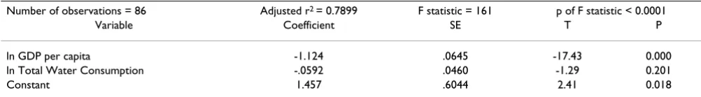
Table 8 shows the results of the best fit regression model for the price ratio of water. The equation fits the data well with an adjusted R squared of 0.79, with an F statistic of 160.79 (p < 0.0001). The coefficient for the quantity of water supplied is not significant in the best fit model. As described earlier, because the dependent variable is a ratio, the elasticity of price with respect to the quantity of water supplied is 1+β (the β is the coefficient of the inde-pendent variable in equation 2). A β of -0.0592 implies an elasticity of 0.9408 – price rises virtually proportionally to the increase in quantity consumed. This suggests either that there are diseconomies of scale, or that the size of the population demanding services allows prices to be increased. On the other hand, price falls slightly with rises in GDP/capita across countries – the elasticity of price with respect to GDP/capita is -0.124.
The best fit regression model for electricity is presented in Table 9. Again, the model fits the data well as judged by the adjusted R squared (0.79) and the F statistic (76.02; p < 0.0001). Unit prices increase with an increase in demand (proxied by consumption) with an elasticity of 0.89 (or 1+ the β coefficient of -0.1098), and with an increase in the percentage of electricity generated from fossil fuel. The elasticity here is almost 2 (1.893) suggest-ing that price increases almost twice as rapidly as the increase in the percentage of fossil fuel electricity sup-plied. Hydropower, nuclear power, or other means of electricity production appear to be lower cost ways of gen-erating electricity than by using fossil fuels.
Price is inelastic with respect to GDP per capita but again the relationship is slightly negative (1 - 1.09 = -0.09), so that countries with higher levels of national income pro-duce electricity at slightly lower unit prices than poorer countries.
Imputing average prices of water and electricity per country
Table 10 reports the estimated values, standard devia-tions, and 95% confidence intervals for the unit prices of water per cubic meter and electricity per KWh for a selected number of countries.
Discussion
The prices of our "non-traded" intermediate inputs vary across countries with variation in GDP per capita, though not always in ways that were anticipated. Prices of printed materials and media advertising increase with GDP per capita. They increase at a slower rate than the increase in GDP per capita, except in Eastern Europe. This suggests that many of the raw materials used to produce these serv-ices are themselves traded internationally, reducing differ-ences in the cost of production across settings. Media in Eastern Europe is an exception, where prices are lower than would be expected for the observed levels of GDP per capita, but they then increase more than proportionally to increases in national income per capita. A possible expla-nation is that some of the governments in the poorer ex-Soviet countries maintain tight control of media outlets which do not yet charge commercial rates for advertising, while the richer countries have been moving more towards a market-based system. Interestingly, the only domestic supply or demand variable influencing price was the size of the population served by media outlets, which seems to allow media companies to charge more because of the increased demand.
On the other hand, there is a negative relationship between the prices of water and electricity and GDP per capita. This would not be expected if market forces played the dominant role in setting prices. Demand, willingness and ability to pay would be higher in richer countries on average, so the lower prices in those settings might repre-sent the use of more efficient, less costly technologies used to produce these services. Another possible explanation lies in the extent of government regulation or control of these markets. It might be that governments in richer countries are more willing, or more effective, in
control-Table 8: Results of regression for price of water in m3
Number of observations = 86 Adjusted r2 = 0.7899 F statistic = 161 p of F statistic < 0.0001
Variable Coefficient SE T P
ln GDP per capita -1.124 .0645 -17.43 0.000
ln Total Water Consumption -.0592 .0460 -1.29 0.201
Constant 1.457 .6044 2.41 0.018
Dependent variable: log ratio of price of water in m3 to GDP per capita. Breusch-Pagan test of heteroskedasticity:1.87 (p Chi2 = 0.17)
ling prices of monopoly producers than those in poorer settings. Alternatively, where governments own the com-panies producing utilities, they might seek to exercise their monopoly powers to extract higher prices more in poorer than richer countries. It is not possible to verify these possible explanations with the data available to us.
In any case, the relationship with GDP per capita is medi-ated by local market conditions reflected in the total con-sumption of water and electricity. Where total
consumption is higher, prices are also higher – higher demand means higher prices, and the marginal cost of production rises with increased output. It also suggests that there are no significant economies of scale which would have suggested a negative relationship with GDP per capita, other things held equal.
Overall, the models fit the data relatively well as judged by the F statistic, R squared, the tolerance test, and visual and mathematical testing for heteroskedasticity. Additionally,
Table 10: Estimated price of water and electricity for selected countries in 2000 I$ and US$
Country GDP per Capita (I$)
In or out-of-sample1
Type Price per unit2 Price per unit
Mean (I$) 95% uncertainty
interval Low
95% uncertainty
interval High
SD Mean (US$) SD
Mali 636 In Water (m3) 1.42 1.15 1.72 0.18 0.45 0.06
Out Electricity (kWh) 0.37 0.25 0.52 0.09 0.12 0.03
Mozambique 720 In Water (m3) 1.37 1.12 1.65 0.17 0.41 0.05
Out Electricity (kWh) 0.26 0.17 0.38 0.07 0.08 0.02
Indonesia 3,168 In Water (m3) 1.13 0.99 1.28 0.09 0.26 0.02
In Electricity (kWh) 0.19 0.15 0.24 0.03 0.04 0.01
Ecuador 3,261 In Water (m3) 1.07 0.89 1.25 0.11 0.36 0.04
In Electricity (kWh) 0.21 0.17 0.25 0.02 0.07 0.01
Algeria 3,949 In Water (m3) 1.35 1.04 1.69 0.20 0.61 0.09
Out Electricity (kWh) 0.22 0.18 0.26 0.02 0.10 0.01
Romania 6,412 Out Water (m3) 1.18 0.97 1.41 0.14 0.30 0.04
Out Electricity (kWh) 0.18 0.16 0.21 0.02 0.05 0.01
Russian 8,036 Out Water (m3) 0.96 0.79 1.15 0.11 0.22 0.02
Federation Out Electricity (kWh) 0.13 0.10 0.17 0.02 0.03 0.00
Bahrain 14,159 Out Water (m3) 1.24 0.83 1.75 0.28 0.98 0.22
Out Electricity (kWh) 0.23 0.18 0.28 0.03 0.18 0.02
Greece 16,706 Out Water (m3) 0.97 0.76 1.19 0.13 0.61 0.08
In Electricity (kWh) 0.18 0.14 0.21 0.02 0.11 0.01
United Arab 20,331 Out Water (m3) 1.26 0.78 1.93 0.35 1.27 0.35
Emirates Out Electricity (kWh) 0.18 0.14 0.22 0.02 0.18 0.02
United 24,348 Out Water (m3) 1.04 0.81 1.30 0.15 1.02 0.15
Kingdom In Electricity (kWh) 0.14 0.11 0.17 0.02 0.14 0.02
Canada 28,088 In Water (m3) 0.78 0.56 1.05 0.14 0.63 0.11
Out Electricity (kWh) 0.11 0.09 0.14 0.02 0.09 0.02
1In and out of sample indicate whether or not the country was included in the data set used to estimate the model. 2Regional estimates are available at http://www.who.int/choice.
Table 9: Results of regression model 2b for price of electricity in KWh
Number of observations = 60 Adjusted r2 = 0.7923 F statistic = 76.02 p of F statistic < 0.0001
Variable Coefficient SE T P
ln GDP per capita -1.090 .0941 -11.58 0.000
ln total electricity consumption -.1098 .0410 -2.68 0.010
ln percentage of electricity generated from fossil fuel .107 .0544 1.97 0.054
Constant .1366 .7399 0.18 0.854
Dependent variable: log ratio of price of electricity in KWh to GDP per capita. Breusch-Pagan test of heteroskedasticity: 2.55 (p Chi2 = 0.11)
contacts in the countries for which out-of-sample imputa-tion was undertaken suggested that the imputed values had face validity.
There are, of course, limitations to the analysis. For exam-ple, we were forced to take data from different countries and different years, deflate or inflate them to 2000, and analyse them as cross-sectional data. This implies that the possible impact of time-related explanatory variables is not captured. While it would have been preferable to use panel data techniques, there were insufficient observa-tions over time and countries to allow this form of analy-sis. Finally, the model is not intended to predict price changes over short time intervals – such as fluctuations in the spot price of electricity – but to impute average prices over a specific time period, i.e., one year.
Policy makers seeking information on the appropriate mix of interventions necessary to achieve their health goals, or the resources required to scale up health inter-ventions, require accurate information. This means that cost estimates should include programme costs, and that the prices used in the calculations should be representa-tive of the range of prices likely to be found in practice. The preferred approach would be to collect a representa-tive sample of observations for each price required for the study, specific to each country, but this is often not feasi-ble or affordafeasi-ble. In this case, we have demonstrated a method in this paper to impute prices for settings where the preferred approach cannot be undertaken, that takes into account variation across and within countries. It pro-duces price estimates that have face validity, and we hypothesize that it is a preferable alternative to basing estimates on a single price observation, or even a few observations, all of which could be outliers.
Authors' contributions
BJ was responsible for data collection, management and analysis, participated in the development of the method-ology and drafted the manuscript. TA contributed to the development of the methodology, as well as data analysis and reporting. DE took part in the development and coor-dination of the methodology and interpretation of the results. All authors contributed to the writing and approved the final version of the manuscript.
Acknowledgements
The authors wish to thank Osmat Azzam, Richard Catto, Yingyao Chen, Gatien Ekanmian, Ruth Lucio, V.R. Muraleedharan, Benjamin Nganda, Sub-hash Pokhrel, Elena Potaptchik, Enrique Villarreal Ríos, Mahmoud A.L. Salem, André Soton, and Lu Ye as representatives of their regional expert teams for their efforts to gather data at the country level. We are grateful to Shakil Ahmed, João Amaral, Debora Gaya, Leslie Mgalula, Chris Mgarura, Mila Montejo, Son Nguyen, George Pariyo, and Ann Ssemogerere for gath-ering additional information for these analyses. Mark Dubner at the Austral-ian Bureau of Statistics provided background information on building costs.
José Hueb provided access to the data on water prices of the WHO and UNICEF Joint Monitoring Programme for Water Supply and Sanitation. Tessa Tan Torres, Rob Baltussen, Dan Chisholm, Raymond Hutubessy, and Chika Hayashi helped oversee the collection of data from the country con-sultants, and Yunpeng Huang helped compile and process the data neces-sary for this exercise. Finally, the former Effectiveness, Quality and Care (EQC) team at WHO and Chris Murray provided general input and feed-back on the development of the methods used. To all, we express our deep appreciation.
The views expressed are those of the authors and not necessarily those of the organization they represent.
References
1. Hongoro C, McPake B: How to bridge the gap in human resources for health. Lancet 2004, 364:1451-1456.
2. Stilwell B, Diallo K, Zurn P, Vujicic M, Adams O, Dal Poz M: Migra-tion of health-care workers from developing countries: stra-tegic approaches to its management. Bull World Health Organ
2004, 82:595-600.
3. Marchal B, Kegels G: Health workforce imbalances in times of globalization: brain drain or professional mobility? Interna-tional Journal of Health Planning and Management 2003, 18:S89-S101. 4. Chen L, Evans T, Anand S, Boufford JI, Brown H, Chowdhury M,
Cueto M, Dare L, Dussault G, Elzinga G, Fee E, Habte D, Hanvo-ravongchai P, Jacobs M, Kurowski C, Michael S, Pablos-Mendez A, Sewankambo N, Solimano G, Stilwell B, de Waal A, Wibulpolprasert S: Human resources for health: overcoming the crisis. Lancet
2004, 364:1984-1990.
5. Baltussen RM, Adam T, Tan Torres T, Hutubessy RC, Acharya A, Evans DB, Murray CJL: Generalized cost-effectiveness analysis: a guide. Geneva, World Health Organization, Global Programme on Evidence for Health Policy; 2003.
6. Adam T, Evans DB, Koopmanschap MA: Cost-effectiveness analy-sis: can we reduce variability in costing methods? Int J Technol Assess Health Care 2003, 19:407-420.
7. Johns B, Baltussen R, Hutubessy RCW: Programme costs in the economic evaluation of health interventions. Cost Effectiveness and Resource Allocation 2003, 1:1.
8. de Jonghe E, Murray CJ, Chum HJ, Nyangulu DS, Salomao A, Styblo K:
Cost-effectiveness of chemotherapy for sputum smear-posi-tive pulmonary tuberculosis in Malawi, Mozambique and Tanzania. International Journal of Health Planning and Management
1994, 9:151-181.
9. CHOosing Interventions that are Cost-Effective [http:// www.who.int/choice]
10. Adam T, Evans DB, Murray CJL: Econometric estimation of country-specific hospital costs. Cost-effectiveness and Resource Allocation 2003, 1:3.
11. Gutierrez JP, Johns B, Adam T, Bertozzi SM, Edejer TT, Greener R, Hankins C, Evans DB: Achieving the WHO/UNAIDS antiretro-viral treatment 3 by 5 goal: what will it cost? Lancet 2004,
364(9428):63-64.
12. Johns B, Adam T, Evans DB: Determinants of variation in health sector wages across countries. Forthcoming 2006.
13. Adam T, Evans DB: Rules of thumb for allocating hospital costs across departments: a multi-country analysis. Forthcoming
2006.
14. Adam T, Ebener S, Johns B, Evans DB: Cost of scaling up health interventions at primary facilities. A multi-country analysis. Forthcoming 2006.
15. Hutton G, Baltussen RM: Valuation of goods in cost-effective-ness analysis: notions of opportunity costs and transferability across time and countries. Geneva, World Health Organization. Global Programme on Evidence for Health Policy Discussion Paper [forthcoming]; 2003.
16. Bade R, Parkin M: Foundations of Macroeconomics 1st edition. New York, Addison, Wesley, Longman; 2003.
Publish with BioMed Central and every scientist can read your work free of charge "BioMed Central will be the most significant development for disseminating the results of biomedical researc h in our lifetime."
Sir Paul Nurse, Cancer Research UK
Your research papers will be:
available free of charge to the entire biomedical community
peer reviewed and published immediately upon acceptance
cited in PubMed and archived on PubMed Central
yours — you keep the copyright
Submit your manuscript here:
http://www.biomedcentral.com/info/publishing_adv.asp
BioMedcentral 19. Gaston N, Doublas N: Integration, foreign direct investment
and labour markets: microeconomic perspectives. The Man-chester School 2002, 70:420-459.
20. Rama M: Globalization and the labor market. The World Bank Research Observer 2003, 18:159-186.
21. Holden S: Wage-setting under Different Monetary Regimes. Economica 2003, 70:251-265.
22. Arbatskaya M, Baye MR: Are prices 'sticky' online? Market struc-ture effects and asymmetric responses to cost shocks in online mortgage markets. International Journal Of Industrial Organ-ization 2004, 22(10):1443-1462.
23. Stata 7: Stata Statistical Software: Release 7.0. College Station, TX, Stata Corporation 2001.
24. Picard RG: A note on the relations between circulation size and newspaper advertising rates. Journal of Media Economics
1998, 11(2):47-55.
25. Brown K, Alexander PJ: Market structure, viewer welfare, and advertising rates in local broadcast television markets. Eco-nomics Letters 2005, 86(3):331-337.
26. Berry ST, Waldfogel J: Free entry and social inefficiency in radio broadcasting. Rand Journal of Economics 1999, 30(3):397-420. 27. United Nations Statistics Division: Advanced data extract. 2003
[http://unstats.un.org/unsd/cdb/cdb_advanced_data_extract.asp]. 28. Seldon BJ, Jewell RT, O'Brien DM: Media substitution and
econo-mies of scale in advertising. International Journal of Industrial Organ-ization 2000, 18:1153-1180.
29. King G, Tomz M, Wittenberg J: Making the most of statistical analyses: improving interpretation and presentation. Am J Pol Sci 2000, 44:341-355.
30. Duan N: Smearing estimate: a nonparametric retransforma-tion method. JASA 1983, 78:605-610.
31. International Energy Agency: Energy prices & taxes – Quarterly statistics [Third quarter 2000]. 2001 [http://www.eia.doe.gov/ emeu/international/elecprih.html].
32. World Energy Council: Pricing energy in developing countries 2001 [http://www.worldenergy.org]. London, World Energy Council 33. Yearbook of statistics. Chronological time series 1992–2001 29th edition.
Geneva, International Telecommunication Union; 2002.
34. Bjornlund H, Rossini P: Fundamentals determining prices and activities in the market for water allocations. International Jour-nal Of Water Resources Development 2005, 21(2):355-369.
35. World Bank: World Development Indicators 2001 Washington, D.C, World Bank; 2001.
36. Countrywatch: Countrywatch information. 2003.
37. Escribano A, Peña JI, Villaplana P: Modeling electricity prices: International evidence. Universidad Carlos III de Madrid: June Work-ing Paper 02-27 2002.
38. Higgs H, Worthington AC: Systematic features of high-fre-quency volatility in Australian electricity markets: Intraday patterns, information arrival and calendar effects. Energy Jour-nal 2005, 26(4):23-41.
39. Knittel CR, Roberts MR: An empirical examination of restruc-tured electricity prices. Energy Economics 2005, 27(5):791-817. 40. Robinson TA: Electricity pool prices: a case study in nonlinear
time-series. Applied Economics 2000, 32(5):527-532.
41. Bottazzi G, Sapio S, Secchi A: Some statistical investigations on the nature and dynamics of electricity prices. Physica A-Statisti-cal Mechanics and its Applications 2005, 355(1):54-61.
42. Borenstein S: The trouble with electricity markets (and some solutions). University of California Energy Institute, Working Paper PWP-081 2001.
43. De Vany AS, Walls WD: Price dynamics in a network of decen-tralized power markets. Journal of Regulatory Economics 1999,
15(2):123-140.
44. Newbery DM: Power markets and market power. Energy Journal
1995, 16(3):39-66.