Bayesian Estimation of the Shape Parameter of the Generalised
Exponential Distribution under Different Loss Functions
Sanku Dey
Department of Statistics St. Anthony’s College Shillong-793001, Meghalaya India
Abstract
The generalized exponential (GE) distribution proposed by Gupta and Kundu (1999) is an important lifetime distribution in survival analysis. In this article, we propose to obtain Bayes estimators and its associated risk based on a class of non-informative prior under the assumption of three loss functions, namely, quadratic loss function (QLF), squared log-error loss function (SLELF) and general entropy loss function (GELF). The motivation is to explore the most appropriate loss function among these three loss functions. The performances of the estimators are, therefore, compared on the basis of their risks obtained under QLF, SLELF and GELF separately. The relative efficiency of the estimators is also obtained. Finally, Monte Carlo simulations are performed to compare the performances of the Bayes estimates under different situations.
Keywords: Bayes estimator, prior distribution, loss functions, root mean square error (rmse), efficiency.
1. Introduction
Let X1, X2, X3, . . . , Xn be i.i.d. Generalized Exponential random variables, with
the shape parameter θ and scale parameter 1, the cumulative distribution function becomes
( ; ) (1 x) ; 0, 0
F xθ = −e− θ x> θ > (1.1)
with the corresponding probability density function (PDF) given by
1
( ; ) (1 x) x; 0, 0
f x θ =θ −e− θ−e− x> θ > . (1.2)
where θ is a shape parameter. When θ=1, the GE distribution reduces to the standard exponential distribution. The GE distribution has a unique mode and its
median is
1 -ln(1-(0.5) )θ .
The rest of the paper is organized as follows. In section 2, we discussed about prior and posterior distribution used in our Bayesian estimation. In section 3, we discussed about loss functions. In section 4, we develop Bayes estimators under quadratic loss (QLF), squared log error loss (SLELF) and general entropy loss functions (GELF) for the shape parameter θ of the Generalized Exponential distribution. Section 5, presents the risk of the Bayes estimators under different loss functions. In Section 6, the efficiency of the estimators is obtained. Numerical experiments are performed and their results are presented in section 7. Finally, the relative efficiency of the estimators is also shown in figures 1- 4 for different values of the parameter.
2. Prior and Posterior Distributions
The Bayesian deduction requires appropriate choice of priors for the parameters. Arnold & Press (1983) pointed out that, from a strict Bayesian viewpoint, there is clearly no way in which one can say that one prior is better than any other. Presumably one has one’s own subjective prior and must live with all of its lumps and bumps. But if we have enough information about the parameter(s) then it is better to make use of the informative prior(s) which may certainly be preferred over all other choices. Otherwise it may be suitable to resort to use non-informative or vague priors (see Uppadhyay et al. (2001), Singpurwalla (2006)). In this paper, we consider that the parameter θ has the non-informative prior distribution and is given by
1
( )
c;
,
0
g
θ α
θ
c
θ
>
(2.1)It is assumed that x=( ,x x x1 2, 3,. . . ,xn) is a random sample from the Generalized Exponential distribution. The likelihood function of θ for the given sample observation is,
n - xi
n
n i = 1 - xi θ - 1
L ( θ | x ) = θ e ( 1 - e ) i = 1
∑
∏ (2.2)
Here, maximum likelihood estimator of θ isn T , with
1 l n (1 ) 1
n x
i
T e
i
− −
= ∑ −
=
.
Combining the prior distribution (2.1) and the likelihood function (2.2), the posterior density of θ is derived as:
( )
(
)
- ( - 1)
-- { ln(1- )-1} - ln(1- )-1
1 1
| ; , 0 ( 2.3 )
- 1
n x n c n x
n c e i e i
i i
x e x
n c
θ θ
π θ θ
+
∑ ∑
= =
which is a gamma distribution with parameters (n – c + 1) and
1
ln (1 )
1
n x
i e i
− −
− ∑
= and the mean of the distribution is
( 1)
1
l n (1 )
1
n c
n x
i e i
− +
− −
− ∑
=
, i.e. ~ (( 1), In(1 ) 1).
1
−
=
−
∑
−+
−c e i
n G
n
i
x
θ
3. Loss Functions
From a decision-theoretic view point, in order to select the ‘best’ estimator, a loss function must be specified and is used to represent a penalty associated with each of the possible estimates. Since, there is no specific analytical procedure that allows us to identify the appropriate loss function to be used, customarily, in most cases for convenience, researchers use the squared error loss function which is symmetrical, and associates equal importance to the losses due to overestimation and underestimation of equal magnitude and obtain the posterior mean as the Bayesian estimate. No doubt, the use of squared error loss function is well justified when the loss is symmetric in nature. Its use is also very popular, perhaps, because of its mathematical simplicity. However, for some estimation and prediction problems, the real loss function is often not symmetric. Asymmetric loss functions have been shown to be functional, see Varian (1975), Zellner (1986). Moorhead and Wu (1998), Spiring and Yeung (1998), Chandra (2001), etc.
Nonetheless, it has been observed that in certain situations when one loss is the true loss function, Bayes estimate under another loss function performs better than the Bayes estimate under the true loss. This serves as a warning to naïve Bayesians who thought that Bayes methods always performs well regardless of situations (see. Ren, et al (2004)). Therefore, we consider symmetric as well as asymmetric loss functions for getting better understanding in our Bayesian analysis.
4. Bayes Estimation
In this section we provide the Bayes estimates of the shape parameter θ based on three loss functions.
4.1. Bayes’ estimator under quadratic loss function (QLF)
In this section we consider the Quadratic Loss Function (QLF)L1( , )θ δ (θ δ- )2
θ
= ,
where δis a decision rule to estimateθ. δis to be chosen such that
θ θ π θ
δ θ
d x
∫
∞
−
0
2
(
θ δ)
qθ xdθ∫
∞
− =
0
2
) /
( , with q( /x) 12 .π(θ/x)
θ
θ =
is minimum. Hereδ =Eq(θ/x).
The Bayes estimator for parameter θ of the Generalised Exponential distribution under quadratic loss function may be defined as
(
)
(
)
0
2 0
1 | ˆ
1 | bq
x d
x d
π θ θ
θ θ
π θ θ
θ
∞
∞
=
∫
∫
n c 1
T
− +
= (4.1)
Where, ln (1 ) 1
1
n x
i
T e
i
− −
= ∑ −
=
4.2. Bayes estimator under squared-log error loss function(SLELF)
The squared-log error loss function is of the form:
(
) (
)
2 1 22 , 1 ln 1 ln ln
L θ δ δ θ δ
θ
= − =
which is balanced with limL2( ,θ δ1)→ ∞asδ1→0or∞. A balanced loss function takes both error of estimation and goodness of fit into account but the unbalanced loss function only considers error of estimation. This loss function is
convex for δ1 e
θ ≤ and concave otherwise, but its risk function has a unique minimum with respect toδ1.
The Bayes’ estimator for the parameter θ of Generalised Exponential distribution under the squared-log error loss function may be given as
[
]
ˆ exp (ln | )
bsl E x
θ = θ
where E(.) denotes the posterior expectation. After simplification, we have
( 1)
1
ˆ n c
bsl e
T
ψ
θ = − +
(4.2)
where,
(
)
(
)
(
1)
1
1
n c n c
n c ψ − + =Γ′ − +
4.3. Bayes estimator under general entropy loss function(GELF)
Calabria and Pulcini (1996) proposed a loss function which is a suitable alternative to the Modified LINEX loss function called a General Entropy Loss Function of the form:
2 2
3( , 2) [( ) ln( ) 1] ; 0; 0
p
L θ δ ω δ p δ ω p
θ θ
= − − > ≠
whose minimum occurs at δ2 =θ. Without loss of generality, we assume that
ω=1.
Following Calabria and Pulcini (1996), the Bayes estimator for parameter θ for the pdf (1.2) under general entropy loss may be defined as
1
ˆ [ ( )]
bge
p p
E
θ = θ− −
provided that E(θ−p)exists and is finite. After simplification, we have
( )
1ˆ p p
bge
K E
T
θ
θ = θ− − =
, where
(
(
)
)
1 1
. 1
p
n c K
n c p
Γ − + = Γ − − +
(4.3)
5. Risks of the Bayes Estimators
The risk of θˆbq under Quadratic loss is
( )
( )
2(
)
(
)
22 2
1 1 1
ˆ ˆ , 2 3 4 3 4
bq bq
R E L n E n E
T T
θ θ δ θ θ
θ
= = − − + −
Since X is a Generalised Exponential variate with parameterθ, then
1 ln(1 ) 1
n xi
T e
i
− − =∑ −
= is distributed asG n
( )
,θ . Therefore, the probability densityfunction of T is given by
( ) ( )
( )
1; ,
0.
n
t n T
g
t
e
t
t
n
θθ
− −θ
=
≥
Γ
Therefore,( )
( )
( )
1(
( ) ( )
)
0 0
( )
.
n
n t
n
E T
t g t dt
t
e
dt
n
n
γ
γ ∞ γ
θ
∞ γ θγ
θ
−
=
−=
− − −=
Γ −
Γ
Γ
∫
∫
Using the above results, we obtain,
( )
2(
) ( ) (
) ( )( )
2 22 1
ˆ 2 1 1
1 1 2
bq
R n c n c
n n n
θ θ
θ θ θ
θ
= − − − + − −
− − −
2
2 ( 1 ) ( 1 )
[1 ]
1 ( 1 ) ( 2 )
n c n c
n n n
− − − −
= − +
− − − . (5.1)
Following the same procedure, the risk of θˆbsl under Squared-log error loss is
( )
(
)
2 21
ˆ ˆ , ( 1) 2 ( ) ( 1) ( ) ( )
bsl bsl
R θ =E L θ δ =ψ n c− + − ψ ψn n c− + +ψ′ n +ψ n (5.2)
Where, ( ) ( )
( )
n n
n
ψ = Γ′
Γ and
1
0
( )n ln y e yy n dy
∞
− −
′
Γ =
∫
is the first derivative of( )n
Γ with respect to n.
and
2
2
( )n d {log ( )}n dn
ψ′ = Γ is the tri-gamma function (see Sinha(1986)).
and the risk of θˆbge under general entropy loss is
( )
(
2)
( 1) ( ) ( )
ˆ ˆ , [ ln 1]
( 1) ( ) ( )
bge bge
n c n p n
R E L p k p
n c p n n
θ = θ δ =ω Γ − + Γ − − + Γ′ −
Γ − − + Γ Γ (5.3)
Note that the above three risk functions are constant with respect to θ as n is known and independent ofθ. Using the Lehmann’s Theorem (1983) [Theorem 2.1 and Corollary 2.1 in section 2 of Chapter 4, pp 249-250], if a Bayes’ estimatorδhas constant risk, then it is minimax, it follows that
2
2( 1) ( 1)
ˆ
( ) [1 ]
1 ( 1)( 2)
bq
n c n c
R
n n n
θ == − − − + − −
− − − ,
( )
ˆ 2 2( 1) 2 ( ) ( 1) ( ) ( )
bsl
R θ =ψ n c− + − ψ ψn n c− + +ψ′ n +ψ n
and
( )
ˆ [ ( 1) ( ) ln ( ) 1]( 1) ( ) ( )
bge
n c n p n
R p k p
n c p n n
θ =ω Γ − + Γ − − + Γ′ −
Γ − − + Γ Γ
are all minimax estimator for the parameterθ of Generalized Exponential distribution under the above mentioned loss functions.
6. Efficiency of the Estimators
In this section, we calculate the relative efficiency of the estimators
ˆ mle
θ ,θˆbq,θˆbsl,θˆbge. where,
1 1
[( ln(1 ) )] ( )
1 1
n x
i
E e E
T n
i
θ
− −
− = =
∑ −
=
and
2
2 1 ( )
( 1)( 2)
E
T n n
θ
=
− −
then,
2
2 1
( )
( 1) ( 2)
Var
T n n
θ
=
Also, we have, 1 ˆ bq n c T
θ = − − and
2 2
2
( 1)
ˆ ( )
( 1) ( 2) bq n c Var n n θ θ = − − − −
The MLE of θ is
ˆ mle
n T
θ = and
2 2
2 ˆ
( )
( 1) ( 2) mle n Var n n θ θ = − − and
(
1)
1 ˆ bsl n c e T ψ
θ = − + and
2
2
2 ( 1)
ˆ
( )
( 1) ( 2)
bsl n c Var e n n
θ
ψ
θ
= − + − − and ˆ bge K Tθ = , where,
(
)
(
)
1 1 . 1 p n c Kn c p
Γ − + = Γ − − +
and
2 2 2 ( 1) ˆ ( ) ( )
( 1) ( 2) ( 1)
bge
n c p
Var
n n n c p
θ
θ = Γ − +
− − Γ − − +
Therefore the efficiency of θˆbqwith respect to θˆmleof θ is 2 1 2 ˆ ( ) 1
ˆ ( 1)
( ) mle bq Var n E n c Var θ θ
= = >
− − , (for n > 1, c≥1 andn> +(c 1)), see figure 1)
Therefore the efficiency of θˆbgewith respect to θˆbqof θ is
2
2 2
ˆ
( ) ( 1)
[ ] ( 1) 1
ˆ ( 1)
( )
bq p
bge
Var n c p
E n c
n c Var
θ θ
Γ − − +
= = − − >
Γ − + , (for n > p and p ≥3, see figure 2)
Efficiency of θˆbsl with respect to θˆbq of θ is
2
3 2 ( 1)
ˆ
( ) ( 1)
ˆ ( )
bq
n c bsl
Var n c
E e Var θ θ Ψ − + − − = =
Efficiency of θˆbsl with respect to θˆbge of θ is
2
4 2 ( 1 )
( 1)
( )
ˆ
( ) ( 1)
ˆ
( )
p b g e
n c b s l
n c
V a r n c p
E
e V a r
θ
θ Ψ − +
Γ − +
Γ − − +
7. Numerical Results and Discussion
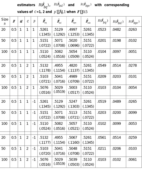
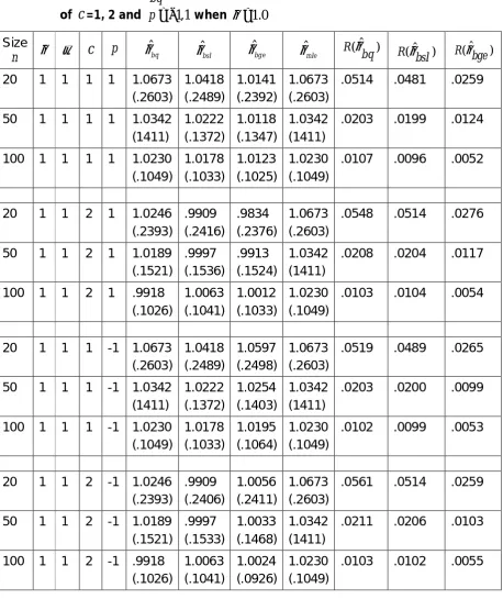
The simulation study considers the performance of Bayes estimation of θ using the prior (2.1) under three different loss functions. The behavior of the loss functions is evaluated on the basis of risk estimates. A comparison in terms of risk values is needed to check whether an estimator is inadmissible under some loss functions. Risks of all these estimators with respect to these three losses have been computed and are presented in Tables 1 and 2. The results of the simulation study are summarized in the Tables 1-2. We simulate samples from (1.2) with the true value of θ = 0.5 and 1, using three different sample sizes (n = 20, 50, 100). All results are based on 10000 repetitions. In the Tables, the estimators for the parameter and the risk, is averaged over the total number of repetitions. Root mean square error (rmse) of each estimate is presented within parenthesis. Tables 1-2 show that under GELF, risk of θˆbge based on non-informative prior is minimum and hence it is admissible for alln,
c
andp. Itis also clear from the tables 1 and 2 that, each of the three Bayes’ estimators has smaller rmse than the classical estimator (i.e., mle) except for the value of
c
=1, when both θˆmleand θˆbqare equal. It is interesting to note that θˆbge withc
=1,p= -1 have smallest risk among all Bayes estimators and the risk of θˆbq with
c
= 2, p= 1 is found to be largest. Further, we note that, the risk of the estimators of θ decreases as n increases.Finally, from the results, we conclude that in situations involving estimation of parameter θ of Generalized Exponential distribution, general entropy loss function could be effectively employed instead of Bayes estimators using a quadratic loss and squared log error loss functions with a proper choice of p . Figures 1-4 shows the relative efficiency of the estimators for different values of
n
,c
and p.Figures 1-4 provide an impression how the efficiencies change with the variation in the values ofn,
c
and p. The figures are drawn using the efficiencies on y-axis and corresponding sample size on x-y-axis. It is observed from figure 1 that as n increases efficiencies decreases. However, the rate of decrease in the efficiency varies for different values ofc
. It is also noted from the results that if the sample size n is sufficiently large then the effect ofc
on efficiencies is negligible. From figure 2, we observe that the efficiency of θˆbgewith respect toˆ bq
Table 1: The Bayes estimatorsθˆbq, θˆbsl, θˆbge, the mle θˆmleand the risk of the estimators R(ˆ )
bq
θ , R(θˆbsl) and R(θˆbge) with corresponding
values of
c
=1, 2 and p= −1,1 when θ =0.5Size
n θ ω
c
p θˆbq θˆbsl θˆbge θˆmleˆ
( )
R bq
θ R(ˆ )
bsl
θ R(ˆ ) bge
θ
20 0.5 1 1 1 .5261
(.1345)
.5129 (.1292)
.4997 (.1253)
.5261 (.1345)
.0523 .0482 .0263
50 0.5 1 1 1 .5151
(.0722)
.5071 (.0708)
.5020 (.0696)
.5151 (.0722)
.0201 .0198 .0102
100 0.5 1 1 1 .5110
(.0524)
.5082 (.0516)
.5054 (.0509)
.5110 (.0524)
.0104 .0097 .0051
20 0.5 1 2 1 .5132
(.1178)
.4955 (.1154)
.4820 (.1137)
.5261 (.1345)
.0549 .0514 .0278
50 0.5 1 2 1 .5103
(.0721)
.5041 (.0716)
.4989 (.0709)
.5151 (.0722)
.0209 .0203 .0101
100 0.5 1 2 1 .5076
(.0516)
.5029 (.0519)
.5003 (.0517)
.5110 (.0524)
.0103 .0104 .0054
20 0.5 1 1 -1 .5261
(.1345)
.5129 (.1292)
.5247 (.1303)
.5261 (.1345)
.0519 .0489 .0265
50 0.5 1 1 -1 .5151
(.0722)
.5071 (.0708)
.5113 (.0721)
.5151 (.0722)
.0203 .0200 .0099
100 0.5 1 1 -1 .5110
(.0524)
.5082 (.0516)
.5057 (.0521)
.5110 (.0524)
.0102 .0099 .0053
20 0.5 1 2 -1 .5132
(.1177)
.4955 (.1154)
.5067 (.1160)
.5261 (.1345)
.0561 .0514 .0259
50 0.5 1 2 -1 .5103
(.0720)
.5041 (.0716)
.5048 (.0708)
.5151 (.0722)
.0211 .0206 .0103
100 0.5 1 2 -1 .5076
(.0516)
.5029 (.0519)
.5039 (.0503)
.5110 (.0524)
Table 2: The Bayes estimatorsθˆbq, θˆbsl, θˆbge, the mle θˆmleand the risk of the estimators R(ˆ )
bq
θ , R(θˆbsl)and R(θˆbge)with corresponding values
of
c
=1, 2 and p= −1,1 when θ =1.0Size
n θ ω
c
p θˆbq θˆbsl θˆbge θˆmleˆ
( )
R bq
θ R(ˆ )
bsl
θ R bge(θˆ )
20 1 1 1 1 1.0673
(.2603)
1.0418 (.2489)
1.0141 (.2392)
1.0673 (.2603)
.0514 .0481 .0259
50 1 1 1 1 1.0342
(1411)
1.0222 (.1372)
1.0118 (.1347)
1.0342 (1411)
.0203 .0199 .0124
100 1 1 1 1 1.0230
(.1049)
1.0178 (.1033)
1.0123 (.1025)
1.0230 (.1049)
.0107 .0096 .0052
20 1 1 2 1 1.0246
(.2393)
.9909 (.2416)
.9834 (.2376)
1.0673 (.2603)
.0548 .0514 .0276
50 1 1 2 1 1.0189
(.1521)
.9997 (.1536)
.9913 (.1524)
1.0342 (1411)
.0208 .0204 .0117
100 1 1 2 1 .9918
(.1026)
1.0063 (.1041)
1.0012 (.1033)
1.0230 (.1049)
.0103 .0104 .0054
20 1 1 1 -1 1.0673
(.2603)
1.0418 (.2489)
1.0597 (.2498)
1.0673 (.2603)
.0519 .0489 .0265
50 1 1 1 -1 1.0342
(1411)
1.0222 (.1372)
1.0254 (.1403)
1.0342 (1411)
.0203 .0200 .0099
100 1 1 1 -1 1.0230
(.1049)
1.0178 (.1033)
1.0195 (.1064)
1.0230 (.1049)
.0102 .0099 .0053
20 1 1 2 -1 1.0246
(.2393)
.9909 (.2406)
1.0056 (.2411)
1.0673 (.2603)
.0561 .0514 .0259
50 1 1 2 -1 1.0189
(.1521)
.9997 (.1533)
1.0033 (.1468)
1.0342 (1411)
.0211 .0206 .0103
100 1 1 2 -1 .9918
(.1026)
1.0063 (.1041)
1.0024 (.0926)
1.0230 (.1049)
Fig.1:Graphs of Relative Efficiency of QL w .r.t MLE for different values of C w hen n=10, 20, 50 and 100
0 0.2 0.4 0.6 0.8 1 1.2 1.4 1.6
0 20 40 60 80 100 120
Sam ple Size
E
ff
icie
n
c
y C=1
C=2
Fig.2: Graphs of Relative Eff iciency of GE w .r.t. QL for diff erent values of C and P w hen n = 10, 20, 50 and 100
0.88 0.90 0.92 0.94 0.96 0.98 1.00 1.02
0 20 40 60 80 100 120
Sam ple Size
Eff
ici
en
cy
C=1, P=1 C=1,P=3 C=2, P=1 C=2, P=3
Fig.3:Graphs of Relative Efficiency of SL W.R.T. QLfor different values of C w hen n=10, 20, 50 and 100
0.82 0.84 0.86 0.88 0.9 0.92 0.94 0.96 0.98
0 20 40 60 80 100 120
Sample Size
Eff
icie
n
cy C=1
C=2
Fig.4:Graphs of Relative Ef ficiency of SL w .r.t. GE for dif ferent values of C and P w hen n=10, 20, 50 and 100
0.84 0.86 0.88 0.9 0.92 0.94 0.96 0.98 1
0 20 40 60 80 100 120
Sample Size
Ef
fi
c
ie
n
c
y
C=1,P=1 C=1, P=3 C=2, P=1 C=2, P=3
Acknowledgements
The author wishes to thank anonymous referee for fruitful comments which led to the improvement of the presentation of the paper. The author also wishes to thank Mr. A.A. Basumatary, Department of Mathematics, St. Anthony’s College, Shillong for his assistance in computations.
References
1. Arnold, B. C. and Press, S. J. (1983), Bayesian inference for Pareto populations. J. of Econometrics, 21, 287-306.
2. Calabria, R. and Pulcini, G. (1996). Point estimation under asymmetric loss functions for left truncated exponential samples. Communication in Statistics-Theory & Methods, 25(3), 585-600.
3. Chandra, M.J. (2001). Statistical Quality Control. CRC Press, Boca Raton.
4. Gupta, R. D. and Kundu, D. (1999). Generalized exponential distribution. Australian and New Zealand Journal of Statistics, 41(2), 173-188.
6. Gupta, R. D. and Kundu, D. (2001b). Generalized exponential distributions: different methods of estimation. Journal of Statistical Computation and Simulation, 69(4), 315-338.
7. Lehmann, E. L., Theory of Point Estimation. New York. John Wiley, (1983)
8. Moorhead, P.R. Wu, C.F.J., 1998. Cost-driven parameter design.
Technometrics, 40, 111–119.
9. Raqab, M. Z. (2002). Inferences for generalized exponential distribution based on record statistics. Journal of Statistical Planning and Inference, 104(2), 339-350.
10. Raqab, M. Z. and Ahsanullah, M. (2001). Estimation of location and scale parameters of generalized exponential distribution based on order statistics. Journal of Statistical Computation and Simulation, 69(2), 109-124.
11. Ren, Cuirong, Dongchu Sun and Dipak K. Dey (2004). Comparison of Bayesian and Frequentist Estimation and Prediction for a Normal Population. Sankhya, 66(4), 678-706.
12. Sinha, S.K. (1986). Reliability and Life Testing. Wiley Eastern Limited. New Delhi, India.
13. Singh, R, Singh, S.K, Singh, U. and Singh, G.P. (2008). Bayes Estimator of Generalized-Exponential Parameters under LINEX loss function using Lindley's Approximation. Data Science Journal, 7, 65-75.
14. Singpurwalla, N.D. (2006). Reliability and Risk: A Bayesian Perspective. Wiley, New York.
15. Spiring, F.A. and Yeung, A.S. (1998). A general class of loss functions with industrial applications. J. Quality Technology, 30, 152-162.
16. Upadhyay, S.K., Vasistha, N. and Smith, A.F.M. (2001). Bayes inference in life testing and reliability via Markov chain Monte Carlo simulation, Sankhya A, 63, p. 15-40.
17. Varian, H. R. (1975). A Bayesian approach to real estate assessment, Studies in Bayesian Econometrics and Statistics in Honor of Leonard J. Savage (eds: S.E. Fienberg and A. Zellner), North-Holland, Amsterdam, 195-208.
18. Zellner, A. (1986). Bayesian estimation and prediction using asymmetric loss function. J. Amer. Statist. Assoc., 81, 446-451.